The Mirage module is a POLIGONSOFT postprocessor designed for visualizing three-dimensional stationary and non-stationary (i.e., time-varying) fields of scalar quantities (e.g., time-varying temperature fields) previously calculated in POLIGONSOFT solvers.
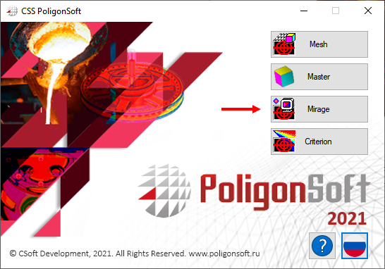
The module is launched from the POLIGONSOFT shell using the Mirage button (see the figure below) or from the "Master" preprocessor by the menu command Simulation → View Results.
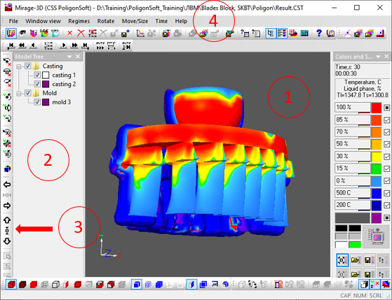
The main part of the module window (see figure below) is occupied by the work area, in which the GM is displayed (1). On the left is the model tree (2), which displays a list of bodies that make up the GM. Toolbars (3) are located on all sides of the module window. The menu bar (4) is also located at the top of the window.
When working with the program, you can use both the main menu commands in the upper part of the window and the buttons on the toolbars. Almost all items of the main menu are duplicated by the corresponding buttons on the toolbars. Further, when describing the functions of the module, their call will be indicated only using the buttons on the toolbars, implying that there are corresponding menu items, as well as hot keys (for some commands) indicated in the names of menu items and tooltips for buttons.
The interface of the Mirage module allows observing the results visually in the form of successively changing temperature, phase and other fields at each simulated moment of time. At the same time, the program provides the standard possibilities of model representation, its scaling, rotation, section, and so on. (see the Common Elements of 3D Modules chapter).
In order to download the required results file, use the buttons located in the upper left part of the window in the Working Commands toolbar, or use the corresponding items in the File menu. All buttons on the toolbars are duplicated by the menu items. The panel has five buttons, each of which opens a file of the results of a certain type.

 |
The button Load the file Temperature loads the files of the type *.CST, containing the phase and temperature fields. You can also use the menu item “File” or key combination Ctrl+T. |
 |
The button Load the file of Porosity loads the files of the type *.P3D to the module that contain the porosity fields. You can also use the menu item “File” or key combination Ctrl+R. |
 |
The button Load the Hydrodynamic file loads the files of the type *.FLW to the module that contain the velocity fields and melt temperatures. You can also use the menu item “File” or key combination Ctrl+F. |
 |
The button Load the Deformations file loads the files of the type *.NDS to the module that contain the stress intensity fields, deformations and movements. You can also use the menu item “File” or key combination Ctrl+S. |
 |
The button Load the universal file loads to the module the files of all above-mentioned types and the files of the universal type *.U3D containing the arbitrary user fields. You can also use the menu item “File” or key combination Ctrl+U. |
After clicking on any of these buttons, the standard file download dialog will appear on the screen, indicating the file to be loaded (see the figure below). If you try to load a file that does not match the selected type, the program will display an error message.
Beginning with the version 15.0, all names of castings and molds can be assigned the names facilitating the navigation in the model tree, in Master and Mirage modules. The names are assigned to the volumes in the Master module and saved to the GM file (*.G3D). Then, when the solvers are started, this information is saved to the results files (except for the hydrodynamic file *.FLW). During loading the results, the Mirage forms the model tree and tries to read the information about the volumes. If the results file is saved by a solver of an earlier version, it does not contain the required information. In this case, a message will be displayed (see the figure below).
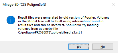
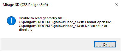
If you click the Yes button, the Mirage will attempt to generate a model tree from the information saved in the GM file of the same name. If there is no file in the folder, or no information is contained in it (the old version of the file), one more message will be displayed (see the figure below) and the model tree will be created based on the information about the volume indices.
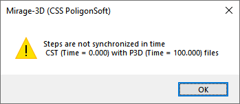
When loading the temperature files, the presence of the same porosity file in the folder is checked. If a porosity file is found, the Mirage checks and synchronizes the simulation steps in the porosity file with the simulation steps in the temperature file. If the information in the files differs, a corresponding message appears on the screen. This means that when viewing the temperatures, simultaneous display of the shrink hole will be impossible.
In the result of loading the module in the working field of the main window, an image of the simulated object will appear, and most of the previously disabled buttons on the control panels will be available. For details on how to control the representation of a simulation object, see the Common Elements of 3D Modules chapter.
 |
The button Model Tree turns the panel with the model tree on in the left part of the window (see the picture below). |
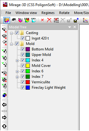
Each volume in the tree has a switch. If you uncheck the box, the selected volume will not be displayed in the working window of the module. When checked, the volume is displayed in the mode specified in the Model Display Modes Toolbar. The same switches have the nodes of the branches ("Casting", "Mold"). If you uncheck the node, all volumes belonging to this branch will not be displayed in the module's working window. Setting a check in the node includes the displaying all volumes of the selected branch.
Each volume in the tree has a color indicator showing the volume index (for more information on the indices of the elements (volumes), see Basic concepts: Volumes, Types, Indices section). For mold volume, the volume index denotes the material. Elements with one material are grouped into the groups, the display of which can also be turned on and off.
 |
The button Notepad with the initial conditions allows viewing and editing the content of the start file *.CFO in the standard application of the Windows – Notepad”. You can also use the File menu or the button F4. |
It is of fundamental importance to understand that the files with the simulation results contain the fields of values of this or that parameters at all points of the modeling object at the moments of the solidification process determined by the specified simulation step. The process of visualization, in essence, is limited to a consistent step-by-step demonstration of these fields in a visual and expressive form. The visibility and the expressiveness of the presentation are achieved due to the powerful device in the program that works with three-dimensional geometric objects, a customizable color palette and the scale of the displayed parameter, as well as a mechanism for controlling the sequence and speed of displaying the simulation steps.
Consider the controls that are responsible for setting up the process of visualizing the simulation results in the work field.
 |
The Palette and Scale Panel button activates the toolbar with the palette, scale and other auxiliary elements and setting buttons in the right part of the working window of the module (more details see in the Palette and Scale section). |
The Mirage module has a control element for visualizing graphic objects – the Palette and Scale panel. (see the picture below). By default, the toolbar is always present on the right side of the window. The menu command Window view → Palette and Scale toolbar is responsible for its display and the button on the working buttons toolbar. The button has the “recess” button when the scale is active.
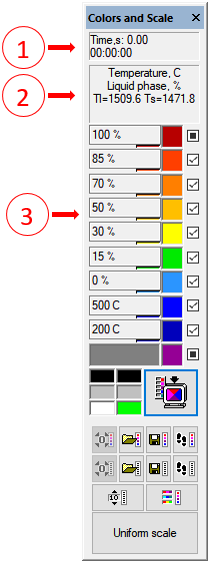
The top part of the panel is occupied by the time counter (1), which shows which moment of the simulated process is reflected in the working field of the module. The time is usually counted from zero, or from the set value of the initial simulation time in the Fourier solver. With the beginning of countdown, the demonstration of the simulation process in the view of color changing zones of the fields of different parameters begins in the working window.
There is the information panel (2) located under the time counter that describes the changes of what parameter is visualized at present moment and how the scale is digitalized itself. Thus when the visualization of the temperature – phase fields is active the scale is digitalized in Celsius degrees and percentage of the liquid phase, and the liquidus and solidus temperature are indicated near used as the references during the simulations. During the visualization of the solidification process in the view of macro and microporosity the scale is digitalized in the percentage of the porosity and so on.
The palette and scale (3) are located under the time counter and the information panel. These two concepts are closely interrelated. The scale is a number of digital values of the visualized parameter. The palette is the colors in which the casting zones (and mold) or their borders will be colored corresponding to the parameters values indicated in this or that point of the scale
The scale has 9 points. The values of the parameter for each point are indicated in its field. The software developers propose the standard scales for different parameters loaded by default as the most illustrative and expressive from their point of view. However, you can customize any of these scales at your own discretion. Clicking the mouse on the parameter value field allows entering it and editing the number indicated there in a usual way. When you edit the scale, for example you can center its points in the zone of parameter changing most interesting for you, to exclude some parameters from consideration and so on. When you edit the scale of porosity, pressure, etc you may not indicate the unit measures. The unit measures set up in the information panel will be used automatically. The exception is the temperature – phase scale because it can have both the temperature in Celsius degrees and the share of the liquid phase in percentage. In order to specify when you are editing that the shares of the liquid phase are meant, you must write the symbol "%" after the entered digit. If this symbol does not exist, the program will automatically read the entered figure as the temperature set in Celsius degrees.
Each point of the scale corresponds to the definite color of the palette. It is visible in a square indicator window to the right of the scale field and on a narrow indicator strip in the lower right corner of the scale field. The presence of two indicators coincides with the fact that the color rendering solution can fundamentally be constructed either on the coloration of the model zones or on the coloration of the boundaries of these zones.
If it is a question of coloring the boundaries, then the colors of the lines of equal parameter values indicated in the scale windows are the colors of the corresponding indicator bars. For example, the line consisting of the points with the temperature 100°C will be the red line, the line consisting of the point with the temperature 200°C – the orange and the line consisting of the points with the temperature 300°C – sharp yellow.
If you use zone coloring, the zones between the adjacent lines of equal parameter values are colored in the color of the indicator window corresponding to the lower of these two parameter values. In the same example, the region of the model having a temperature of 100 to 200°C will be colored red, and the region of the model having a temperature of 200 to 300°C will turn orange.
The software developers propose the standard palettes for different parameters loaded by default as the most illustrative and expressive from their point of view. Thus, the standard temperature-phase palette is built on the transition simulating the cooling of the metal: from white through red to blue, the palette of porosity - on the transition from the black color of shrink heads to the white color of an absolutely non-porous metal, the pressure palette is sustained in the blue scale and the intensity of staining in it corresponds to the growth of pressure
However, you can customize any of these scales at your own discretion. Clicking the mouse on the palette color indicator marks it with a tick and opens the standard window for Windows applications "Color", in which you can select any color available to your computer in a known way. After closing the window with the OK button, the selected color will be assigned to the current palette indicator.
To the right of each indicator there is a checkbox for fixing the color (or value). When it is set, the color (or value) assigned to a specific point on the scale does not change, depending on the state of the neighboring points of the scale. If the check box is cleared, then the color (or value) of the "marked" indicator is automatically set intermediate between adjacent states of the scale. We draw your attention to the fact that the checkboxes of fixation from the extreme color indicators cannot be removed, which is emphasized by the pale drawing of these checkboxes. To better understand the specifics of working with the palette and the values of the scale, we advise you to experiment with it yourself.
Each field type (temperature, porosity, pressure and so on) has its own scale and palette. The last used palette and scale of each type is remembered and used in next sessions of the software work (the current palettes and scales are being saved automatically to the disc and read during the next start of the program).
 |
If you have changed the scale or the palette and want to apply them to the image in the working field, you need to press the Apply Colors and Scale button. This button is located above the scale, exceeds all other buttons by the size, and becomes available after making any changes to the scale or palette. This is indicated by the coloring of the icon on the button. |
Under the Scale and palette enter button there are two rows of the same buttons, the upper one refers to the palette, and the bottom - to the scale. If to consider them in pairs, the buttons have the same functionality:
  |
The buttons Standard palette (all colors) and Standard scale restore the standard palette and scale accepted by default. |
  |
The buttons To read the scale palette and To read the scale open the standard file load window to find on the disc and to load the scale (SCL) or palette file (PAL) previously saved. |
  |
The buttons To save the scale palette and To save scale open the standard save window in which you can save as the file the current scale (SCL) or palette file (PAL) in any place desired on the disc. |
  |
The buttons To restore the palette (all colors) and To restore the scale cancel the last changes entered to the scale or palette. |
Below there is one more row of the control buttons for the scale and palette:
 |
You can enter the numbers for the whole scale or a part of it setting the step between the scale values. To do it you need double click the button Step for the Scale. After that the dialog panel will be called for editing the scale with the help of the specified step (see the picture below). |
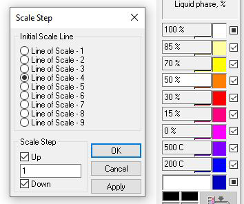
In the Initial Scale Line group with the help of radio-buttons it is necessary to specify what value of the current scale will be decided as the reference point. This value of the scale will stay without changes and all other values above and (or) below indicated will be changed in accordance with the specified step. When choosing the initial scale line with the help of the radio-buttons the corresponding value will be simultaneously highlighted on the scale itself.
In the Scale step group it is necessary to specify the step and with the help of the checkboxes Up and Down to indicate whether it is necessary to change the scale below or above the indicated initial line or not. Clicking the Apply button you can enter the new values to the scale not closing the dialog panel. If to click the Enter button then the new values will be entered to the scale and the dialog panel will be closed. To cancel the scale edition you need to click the Escape button or the crisscross in the right upper corner of the dialog panel (or the button Esc).
 |
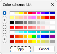
To set the color palette you can use the list of the standard color schemes that is called by the clicking the Color Schemes button. Color schemes List dialog will be opened in which with the help of radio-buttons you can choose one of the ready color schemes of the palette (see the picture below). The scale will be applied after clicking the Apply Colors and Scale button. |
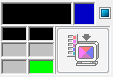
Using the Palette and Scale toolbar you can adjust the background color of the working field and three service colors used by the program for contour the lines, meshes, arrows of axes and other auxiliary images. The adjustment is the same as setting the palette. The indicators of these colors are located on the left and on the top-left of the button "Entering the Scale and Palettes" (see the picture below).
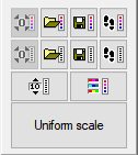
At the bottom of the scale of the Mirage module there is a Uniform Scale button (see the figure below), which is used to quickly adjust the scale for the maximum and minimum field values in one click.
In the Mirage module, along with the already familiar image control buttons (see the 3D Modules Window View section), there are several additional buttons on the visualization mode panel (see the figure below).

Switching of color decisions of the visualization of the simulated fields is carried out by two buttons located on the mode panel.
 |
The Visualization mode of the color regions button switches on the mode of zone coloring of the simulation area on. In other words, in this mode (it is active by default) the geometry is represented as 3d or 2d areas of the area, colored according to the settings of the palette, the scale and some other settings. |
 |
The Visualization mode of the color isolines button switches on the mode of boundary coloring of the simulation area on. In this mode, the geometry is represented as a set of isolines, colored in accordance with the settings of the palette, the scale and some other settings. |
To the right, on the same panel there is a group of buttons responsible for visualizing the results of stress simulation. The following buttons become active when the "deformation file" *.NDS is loaded into module.
 |
The Show the stress fields button switches on the mode of visualization of the stress intensity on. |
 |
The Show the deformation fields button switches on the mode of visualization of the deformation intensity on. |
 |
The Show the deviation fields buttons witches on the mode of visualization of the values of the movement vectors of the mesh nodes of the geometric model. |
 |
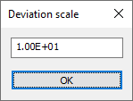
The The scale factor of the deviation field button allows you to set the coefficient by which the components of the movement vector are multiplied at all mesh nodes. This allows the user to see even a slight warpage of the casting. In this case, the field values (for example, the deviation fields) are displayed in true units, scaling only affects the visualization of the geometry. The default factor is 10 (see the figure below). |
 |
The Show the cracks button switches on the visualization of the nodes on, in which the stress intensity values exceeded the specified strength (for the current temperature in the node). |
One more tool for visualization the simulated fields is the kinetic isolines. In part, they are similar to the isosurfaces (see the description of the isosurface modes below); however, they have two important differences:
Control of the kinetic isolines is carried out using a group of three buttons on the Modes Panel.
 |
The Create the kinetic isolines button serves for the generation of the lines with the equal at a given time the simulation values of the displayed parameter. Clicking on it opens the Kinetics (Create) window (see the figure below), which contains a list of parameter values allowed for constructing the isolines. |
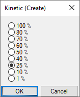
Note that the list of allowed parameter values coincides with the parameter values assigned to the reference points of the scale in the palette and scale bar. The choice of the parameter value, for which an isoline is to be built, is carried out using the radio buttons. Pressing the OK button starts the generation of isolines, and pressing the Cancel button closes the window.
 |
The Kinetic Isolines Parameters button allows to specify the time parameters for demonstrating the isolines. Clicking on it opens the Kinetics (Show) window, where you can use the radio buttons group to select the step frequency of the isolines display, and use the checkboxes to define the time interval for simulation, within which the isolines will be saved in the model image (see the figure below). |
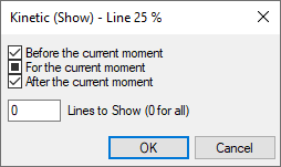
The For the current moment checkbox is not removed; because this isoline is always displayed on the model. The Before the current moment checkbox assumes the saving all isolines from its start of a step-by-step demonstration to the current time. The After the current moment checkbox assumes the successive erasure of all isolines from the beginning of the step-by-step demonstration to the current time (At the same time, the isolines stay on the model, simulated as if with the anticipation at the end of the simulation.)
Pressing the OK button confirms the acceptance of the set parameters, and pressing the Cancel button closes the window without changing the parameters.
 |
The Kinetic isolines On/Off button controls the output of already generated isolines to the screen directly. It also turns on the contours of the cutting plane and the sections, if those were not included by the corresponding buttons on the mode toolbar. |
In addition, a few more buttons on the visualization mode panel control the visual representation of the simulation object in the working field.
 |
The Melt mirror On/Off button shows the current location of the melt mirror. The mirrors are shown in the form of green flat meshes. Note that the mesh that visualizes the mirror is formed by intersecting the plane of the mirror and the faces of the finite elements of the local feed zone in which this mirror is located. Thus, the mesh of the mirror does not accurately show the edges of the mirror; these edges can also pass inside the element (if the part of the element has already solidified). The command is available when viewing the results of simulation the porosity (file *.P3D). |
 |
The All Mirror Mirrors On / Off button displays simultaneously all positions of all melt mirrors that have been saved in the results file of the porosity simulation *.P3D. |
 |
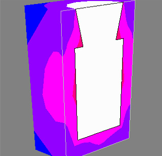
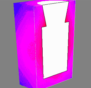
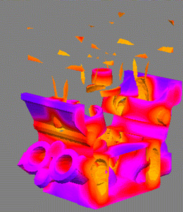
The Smooth Color Transitions On / Off button controls how to color the image areas corresponding to the different points on the scale. If the button is pressed, then between the adjacent zones a smooth color transition is realized without an explicit boundary, otherwise the zones have the clear boundaries, and each of the zones is colored by its monotone color, regulated by the adjustment of the scale and the palette. Examples of the visualization are shown in the figures below. |
 |
The Dynamic Environment On / Off button controls the display of the dynamic environment (if it is used in the simulation). When the button is pressed, its current location (the environment) and the temperature of the layers are displayed (see the figure below). |
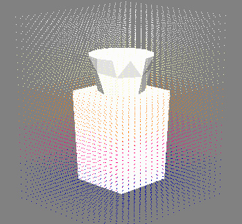
The dynamic environment is visualized as the moving points relative to the base GM, the color of which corresponds to the current temperature of the given point of the environment in accordance with the settings of the palette and scale.
 |
The Moving the geometry in radiation simulation On / Off button allows you to visualize the area of simulation of the radiation (shown in dashed lines) - some dimensional rectangle, as well as the movement of the geometry elements relative to each other (see the figure below). |
In the Mirage module, several additional buttons appear on the mode toolbar for the casting and the mold (see the figure below) along with the already familiar the casting and the mold control buttons (see the Model Display Modes section).

In the button groups related to the casting and mold display, there are three additional pairs of the buttons.
  |
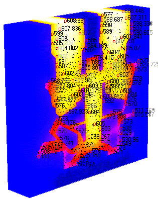
The Digitizing Casting Section On/Off and Digitizing Mold Section On/Off buttons turn on and off the indication of the values of the simulated fields (temperature, porosity, voltages, etc.) at various points of the section of the model. In this case, the point to which the numerical value of the field refers is indicated on the model by a colored circle (see the figure below). |
The density of the location of the points on the image is automatically selected in such a way that the displayed numbers do not overlap each other. Therefore, as the image is magnified in the working field, the absolute number of the digitized points increases.
  |
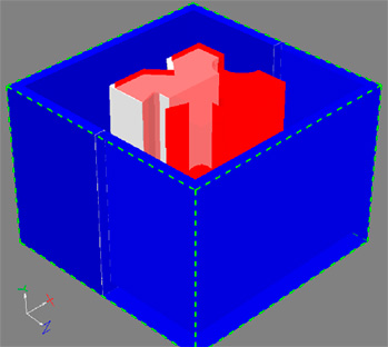
The Transparent Casting On / Off and Transparent Mold On / Off buttons enable and disable the mode of displaying the semitranslucent casting and the mold volumes. The mode improves the perception of the information when viewing the filling of the casting volume or in the modes of the isosurface display, i.e. in those cases when the parts of the volume are not filled with the material. |
  |
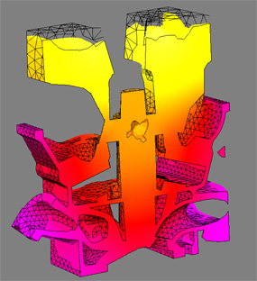
The Casting Isosurface and Mold Isosurface buttons serves to display the geometry in the form of surfaces with the equal values of the parameter being visualized at a given time of simulation. Clicking on them opens a dialog box with the display settings (see the figure below). |
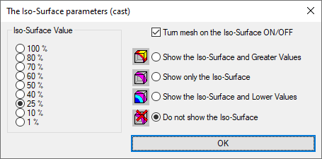
In the left part of the window, there is a list of the values of the parameter allowed for constructing the isosurfaces. Note that the list of allowed parameter values coincides with the parameter values assigned to the reference points of the scale in the palette and scale bar (see the Palette and Scale section.)
The choice of the parameter value, the isosurface for which it is necessary to build, is carried out with the help of a group of radio buttons. To the right of the window there are the radio buttons for selecting the isosurface representation:
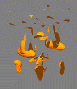
The Isosurface Mesh On / Off option at the top of the window allows you to apply a mesh of finite element faces to the isosurface.
The "Enter" button at the bottom of the window starts the isosurface generation process, after which the image is converted appropriately in the working field. It should be emphasized that the isosurfaces are generated for all simulation steps and the results of the step-by-step demonstration of its results undergo corresponding dynamic changes.
 |
The Show Shrinkage Pipes button turns the display of holes on when viewing the casting temperature and phase fields (*.CST file). The command is available if the CST file is opened and the same file with the results of porosity simulation (*.P3D) is in the same folder as the *.CST file. |
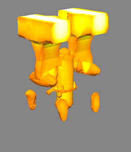
If the above conditions are performed, the “Show shrink holes” command becomes available. When the button is clicked, the Mirag module reads the porosity information from the *.P3D file and turns on the Show the isosurface and below geometry display mode with a porosity threshold value of 50%. Thus, the shrink holes are displayed on the current geometric model (see the figure below).
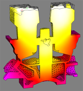
The display of the shrink holes is, in essence, a mode of showing the isosurface, but it does not limit the modes of displaying the temperature and phase fields. The figure below shows the operation of the isosurface mode for the temperature field simultaneously with the Show Shrinkage Pipes function.
 |
The Velocity field button shows the Parameters of the velocities field dialog (see the figure below) in which you can adjust the parameters of displaying the velocity field in the vector form. The command is available if the melt flow simulation results file *.FLW is open. |
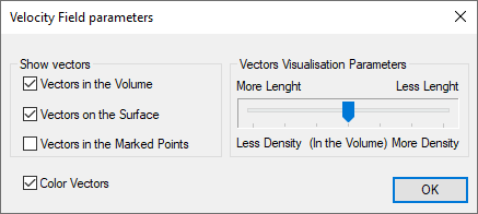
In the left part of the dialog box, there are the checkboxes that control the switching the display of the vectors in the volume on, on the surface and / or in the previously marked points of the simulation area. On the right, there is a slider controlling the frequency of the arrows of the vectors. The display algorithm is configured so that the more number of vectors the user wants to see on the screen, the smaller their length and vice versa. At the bottom of the dialog, there is the Color vectors checkbox, which includes the coloring of the vectors in accordance with the given scale and the palette of the velocity of the flow. The ОК button confirms the settings used. If at least one of the methods of displaying the vectors is selected in the left part of the window, then after pressing the OK button and closing the dialog, the Velocity field button will accept the recessed position (the vectors are shown). If all checkboxes of the Show the vectors group are removed, after pressing the ОК button and closing the dialog, the Velocity field button will be turned off (the vectors are not displayed).
Let's consider a group of buttons that forms the Time Control panel, which by default is placed on the upper part of the working field on its right side (see the figure below). To call or to hide this panel, if necessary, you can use the Time Control Bar comand in the Time menu.

The Time Control panel is designed to specify, in one way or another, the simulation time point, which is visualized in the working field. Six buttons, combined in two similar groups, resemble the buttons of the player. Clicking on them provides the movement from the current simulation step:
  |
To the first and last simulation step correspondingly; |
  |
Five steps back or five steps forward correspondingly along the simulation time axis; |
  |
To the previous or next step of the simulation. |
 |
Between these groups there is the Time Scale button, which allows you to go to any step of the simulation. Clicking on it brings up the Select Time dialog box (see the figure below). |
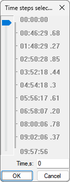
The central part of the window is occupied by a time scale with a slider, digitized according to the time parameters saved in the open file. At the moment of the window opening, the slider is in the position corresponding to the current time of simulation. To go to the simulation point of interest, you should set the engine to the appropriate position. In this case, the value of the selected time in seconds will be displayed in the Time field located below. With this field, you can also set the required moment of time directly in the numerical form. To do this, simply place the cursor in the field, enter the desired time in seconds from the keyboard and press the Enter key on the keyboard. In this case, the slider will occupy the corresponding position on the scale. Note that if a too long time value is entered, then the final simulation time will be automatically set in the field. Pressing the OK button confirms the selection of the time moment and leads to the appearance of the corresponding picture of the simulated field. Pressing the Cancel button closes the window without changing the displayed time point.
The procedures described above allow one to observe the discrete states of the solidification process. However, in the Miragemodule there is the possibility of a dynamic representation of the process.
 |
The Autoview of time steps On / Off button starts the mechanism of the sequential change of model images in the working field. The starting point of step-by-step visualization is the current time in the working field, regardless of how it was assigned. |
 |
You can set the mode of automatic and / or manual viewing using the Time step parameters button. Clicking on it opens the Time control parameters dialog box (see the figure below). |
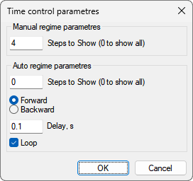
The window is divided into two parts. At the top there is a field in which the number of skipped steps is specified when viewing with the or buttons. Thus, to view every fifth saved step in time, you need to set this field to 4 (four steps will be skipped, the fifth will be shown).
Below there is a group of elements of automatic view control. There is a similar parameter. In both cases, setting this field to "0" means that all saved steps will be displayed.
Two radio buttons located in the group of elements of automatic view control make it possible to set the direction of the auto review:
In the Delay field you can set the changing frequency of the successive steps of the visualization. To do this, enter the desired delay time in the field between the steps in seconds.
Setting the Loop checkbox allows you to organize an "in a circle" view, i.e. after the last step is shown, the demonstration will begin again.
Pressing the OK button confirms the specified parameter settings. Clicking on the Cancel button closes the window without saving the changes.
It is necessary to add that changing the parameters of automatic viewing is possible directly in its process.
The Mirage module allows you to view and to analyze the simulation results directly during its execution.
 |
The Hold the last step button turns the mode of tracing changes on in the current file results, opened in the module. |
When using this mode, the last saved simulation step is permanently displayed in the working window of the module. During the simulation, the solver modules save the results of the simulation to files with a specified frequency. With the Hold the last step button pressed, the Mirage module monitors the appearance of new records and automatically loads them. Thus, the user always sees the current status of the simulation on the screen. The function is especially useful in simulating the fill and stresses, i.e. in those cases where solvers do not have their own visualization tools.
When describing POLIGONSOFT, the terms "two-dimensional" and "three-dimensional" terms are used repeatedly and without any special comments. This means the plane or the space of the simulation object for which this or that simulation is performed. But in reality for each point of a two-dimensional or three-dimensional object in the results of a dynamic simulation there is another coordinate, in addition to the spatial coordinates. This coordinate is time. It is obvious that for each point it is possible to visualize the change in some function (for example, temperature) in time in the form of a graph.
In addition to the temperature, in the results of the simulation of POLIGONSOFT other functional dependencies can be met. Thus, for a static field of porosity, for example, it is possible to visualize a change in porosity over the height of the casting.
The methods of the visualization of the curves (graphs) are described further in the section Visualization of the curves (Mirage-L module).
 |
For generation, use the Create a graphics file for a point button located on the working buttons panel. Initially this button is not active, i.e. is not available for use, because no model points have been defined for which graphics files will be generated. |
To set the point (s) for which the curves will be made, just point the cursor at the desired place of the object, and double-click the left mouse button (see the figure below).
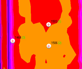
In the working field, the point is displayed as a white ball with a crosshair. Next to it the current value of the visualized field and the serial number of the point (green in parentheses) is displayed. A point can be placed on any visible part of a geometric object, be it its surface or section. In the figure above, the temperature field values are shown as an example. When using the time control buttons (forward, back, etc.) and moving through the simulation steps, the values at the selected points change and show the actual information. To remove a point, you must point the cursor at it and double click with the right mouse button. You can remove all points by combining hot keys Ctrl+D.
After you have defined one point at least, the Create a graphics file for a point button becomes available. Clicking on it opens the Graph Type dialog box (see the figure below).
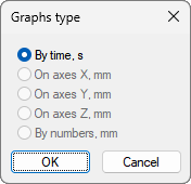
In this window, using the radio buttons, you can choose one of the following graphs options:
By the time, sec – the abscissa represents the process time, i.e. plotting the curve of the time-field values;
Along the X axis, mm – the value of the X coordinate is plotted on the abscissa, i.e. a curve is made for the value of the field along a line parallel to the X axis and passing through the selected point;
Along the Y axis, mm – the value of the Y coordinate is plotted on the abscissa, i.e. a curve is made for the value of the field along a line parallel to the Y axis and passing through the selected point;
Along the Z axis, mm – the value of the Z coordinate is plotted on the abscissa, i.e. a curve is made for the value of the field along a line parallel to the Z axis and passing through the selected point;
By numbers, mm – a curve is constructed for changing the value of the field along a broken line drawn from the point to point in accordance with their ordinal numbers.
Pressing the OK button starts the generation of the corresponding file or the files. Clicking on the Cancel button closes the window without generating the file (s). At the end of the generation process, the standard Windows application window will be opened, where you will enter the files and choose the place to save them. The graph files in the POLIGONSOFT have a LIN extension
 |
The View the Graphics files button loads the Mirage-L module in which the demonstration of the created curves is performed. To start the module you can use the combinations Ctrl+L. The visualization methods of the curves (graphs) are described further Visualization of the curves (Mirage-L module). |
At one given point and choosing the type of the By time curve, a graph of the time dependence of the displayed parameter for a given point is created. If several points were specified, the program generates the separate files for each point, adding "_ (point number)" for each of them to the end of the given name.
When you select the type of the curve Along the axis... a gradient graph of the displayed parameter is created in the selected direction without taking into account the sequence numbers of the points. Obviously, in this case, the definition of one point is not enough, and at least two points should be determined. Regardless of the number of certain points in this case, one file is generated.
If you select the type By numbers, you create a graph similar to the gradient of the displayed parameter along the axis. However, an essential difference of this graph is that the abscissas of the points on it are not the coordinates along the axis, but the absolute distances between the points, taking into account their ordinal numbers. Obviously, in this case, the definition of one point is also not enough, and you should determine at least two points. Regardless of the number of certain points, in this case one file is generated.
All points that are put in order to find out the value of the fields in them or to create the curves for these points can be saved to a separate file. Subsequently, you cannot generate these points again, but download them from this file. This can be extremely convenient when analyzing a certain place in the same casting, but simulated according to the different regimes or with different elements of the intake system.
 |
The Create the file with the defined points button allows saving the created points in the files with the extension PNT. The button is located on the working buttons panel. |
 |
The Load the defined points from the file button loads the PNT files to the previously saved points. The button is located on the working buttons panel. |
When viewing the fields saved in hydrodynamics (FLW) files, you can observe how the cavity of the mold is filled. Thus, in the process of filling, the 3D geometry of the casting changes. The Mirage module provides the ability to save any stage of filling into a separate 3D geometry file in the POLIGONSOFT geometry format (G3D).
 |
The Create the file with the current geometry button creates a file of geometric model G3D, focusing on the current mold filling state. The button is only active when viewing the fields from the hydrodynamic files (FLW). |
After that, you can work with this geometric model (3D mesh) as with the conventional finite element geometry: edit in the Master module, perform the simulation in the Fourie and other solvers, etc.
Another tool provided in the Mirage module is the creation of the files of two-dimensional fields of the displayed parameters. These files are created by sampling from the results of three-dimensional simulations of those parameter values that relate to the current section of the model.
 |
The Create the file of 2D-fields button creates the files containing the simulation results (field value) for the selected section of the casting and/or the mold. |
It is possible to create the following files of 2D-fields:
ANT – the thermal fields of the casting (the enthalpy field, over which it is possible to recover the temperature and the fraction of the solid phase);
TMF – the temperature fields of the mold;
POR – the fields of macro- and microporosity;
UNI – the universal fields.
When simulating the stresses and the deformations in a casting without taking into account the contact interaction with the mold, it is necessary to set the special boundary conditions for some mesh nodes - the fixing conditions. The purpose of the fixing conditions task is to exclude the possibility of the movement of the entire casting as an absolutely rigid body. Otherwise, the task turns out to be undetermined, and the movement field acquires a certain degree of arbitrariness (the corresponding elastic-plastic task has an infinite set of solutions). This can lead, in particular, to the fact that at each step of the simulation the part will be moved or rotated in an unpredictable manner, or even to the impossibility of stress simulation on the individual simulation steps.
The fixing conditions task can be performed either automatically or manually. A detailed description of the principles of fixing is described in the corresponding section Nodes Fixation, here you will find the tools necessary for this operation.
The points (nodes) for fixing the geometry are defined in the special mode of the module Mirage - The boundary conditions setting mode. To enable it, the Boundary conditions toolbar menu should be selected in the Window View menu, which makes the toolbar of the same name visible (see the figure below). In addition, it is required that the CST casting temperature field file is loaded.

 |
The Boundary conditions setting mode button turns a special mode on for marking the mesh nodes and imposing the restrictions on the movement of these nodes along the coordinate axes. |
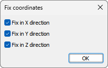
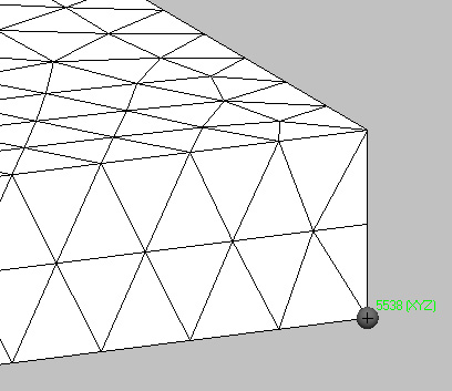
When the Boundary conditions setting mode button is turned on, double-clicking on the geometry with the left mouse button, the node closest to the mouse pointer is found and the Fix coordinates dialog opens (see the figure below).
Note. In this situation, it is convenient to turn the mesh casting mode on.
By marking the necessary positions with the tick marks, the movements of the selected node along the coordinate axes is fixed. After pressing the OK button, the selected node is marked on the geometry of the casting with a dark gray ball (see the figure below). Near the mark, the node number is written in green, the coordinates along which the movement of the node is forbidden are indicated in parentheses (the node is fixed).
After the required fixing scheme is created, i.e. the nodes are selected and their movements are fixed, you can save this scheme to the MCST boundary condition file. This file can then be used in the Hooke module (if using the "manual" mode of fixing the geometry).
You can restore the fixation pattern at any time by uploading the CST file to the Mirage module, and then downloading the file of previously saved MCST boundary conditions.
The operations for saving and loading the MCST file are saved by the following commands on the Boundary conditions panel:
 |
The Create the boundary conditions file button opens the standard Windows dialog for saving the MCST file. |
 |
The Load the boundary conditions file button opens the standard Windows dialog for loading the MCST file. |
The demonstration of the results of the simulation in the form of video clips is a rather effective technique. First of all the advantage of showing the video before the demonstration of the process using the automatic viewing, is that the video can be played on any computer. You do not need to install a postprocessor; you do not need to download the results files, which are usually large (hundreds of megabytes or gigabytes).
 |
The Save the video button allows creating the video – files in the AVI format. Pressing this button opens the standard save window in which you need to choose the place of saving and to write the name of the file. |
After entering the name, the Video file recording parameters dialog box opens (see the figure below). In the upper part of the window, you need to specify the length of the video. It can be set either directly in seconds, or indirectly as a frame rate. To do this, select the appropriate switch (radio button) and enter the value of the selected value in the adjacent field.
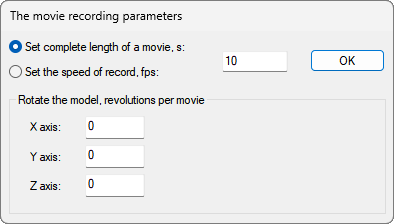
For example, if you intend to record a video of the process of melt pouring into the mold, you can select the Set the total length of the film switch and enter the fill time of the mold. In this case, you will get a file showing the process in time close to the real.
At the bottom of the window, there are the fields in which you can set the rotation of the model during the video recording around the three coordinate axes. By default, the corresponding fields are set to "0", which means the model is stationary. If you enter some values in these fields, the geometry will rotate when the movie is saved. The speed of the rotation is determined by the preset length of the video and the entered number of complete rotations around the axes. You can specify the simultaneous rotations around all three axes.
After entering the necessary parameters for video recording, you should click the OK button and go to the next dialog Video Compression. Here you can specify the video compression program and choose the compression quality. By default, the recording of full frames without compression is set. This means that the quality of the video image will be the best, and the file will have the maximum size.
If desired, you can select one of the codecs from the list found in the system and adjust the quality of the compression using the slider Compression quality. In addition, you can use the Configure ... button (if it is active) to go to the codec settings window.
Pressing the OK button starts the video recording, pressing the Cancel button will cancel the process.
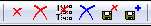
The Mirage postprocessor has a functional that allows you to edit the results files (CST, P3D, NDS, FLW, etc.). The commands responsible for editing the files are grouped in the Working Commands panel (see the figure below).
Basically these operations allow you to delete some records of the results from the files and thereby to reduce their size.
 |
The Cut the current step button marks the current simulation step for deleting the results from the file being viewed. The command can be executed by pressing the Del key on the keyboard. At the same time, a red cross is displayed in four corners of the working window, similar to the icon on the button (see the figure below), and the button remains turned on (recessed). |
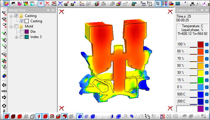
When viewing the simulation steps and passing through the steps marked for deletion, these characters will be displayed, and the "Cut the current step" button will be automatically turned on. Any step marked for removal can be restored by pressing the button again (in the recessed state it is called Return current step), or by pressing the Del key on the keyboard again.
In some cases, it is easier to mark the steps that need to be left, i.e. you need to delete all steps except some.
 |
The Delete all steps button marks all simulation steps of the viewed results file for deletion. The button itself becomes inactive. When viewing any simulation steps, a red cross is displayed in four corners of the working window, similar to the icon on the Cut the current step button, and the button itself remains always on (recessed). |
Since deleting all steps from the simulation in terms of the same as deleting the file itself, it is understood that after using the "Delete all steps" button, the user will find the steps that need to be saved and restored by clicking the "Return the current step" button.
 |
The Restore all steps button restores all steps marked for deletion of the results file being viewed. The button itself becomes inactive. When viewing any simulation steps, a red cross is displayed in four corners of the working window, similar to the icon on the Cut current step button, and the button itself remains always on (recessed). |
Above we considered quite simple cases of deleting the simulation steps. To perform more complex operations, for example, to remove the n-th number of steps every m steps in an arbitrary range (starting with step i, but no further step j), a special tool is used.
 |
The button Cut / Restore the random steps opens the dialog box with the same name, where you can flexibly manage the process of deleting the simulation steps (see the figure below). |
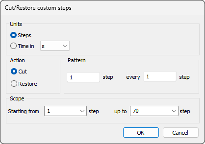
In the Units block, on the basis of what criterion the removal of the steps from the file will be performed. In fact, it specifies the units in which all other parameters in the window are specified.
In the Action block, you should specify what action (delete or restore) is being performed at the exact moment. In the Pattern block, you specify the order of the procedure, which is determined by two numbers: each what step to perform the action and after how many steps to repeat it. For example, if the delete mode is selected, then entering the number in the step field is 5, and in the field every ... step the number 10 is as follows: 5 steps will be deleted, then 10 steps are skipped, then 5 more steps are deleted, etc. It should be noted that the first step always remains (you can consider it to be zero).
In the Scope block, the range of steps in which the delete or restore operation is performed is specified. You cannot delete steps in all simulation, but only in a certain part of it. The beginning and the end of the range are specified in the fields Starting from and Up to ..., respectively.
After you have set the rule for deleting or restoring the steps, you should click the OK button to apply the rule or Cancel to refuse the action.
Check how the marking of the steps for deletion or restoring is performed using the time scale, i.e. scrolling the process forward or backward and observing the steps marked for removal.
To mark the steps for deleting does not yet mean, in fact, to cut them from the file. The Mirage module monitors the safety of the user data, so a special command is executed to complete the step removal operation.
 |
The button Save a file without marked (cut) steps opens a standard file saving dialog where it is suggested to specify a new name for the file with the cut out steps. The file name [open file name]_cut with an extension of the appropriate type is automatically offered. |
Thus, writing a new file without the deleted steps does not affect the original file. The user can pre-test the result of the deletion in the Mirage module, and then decide whether to delete the initial file from the disk or not. Of course, if you save the cut file with the selected name of the initial file, the system will ask for confirmation to overwrite. If the user gives the appropriate permission, the original file will be replaced with a new one.
In addition to the editing method described above, the Mirage module has the ability to merge two files of the same type. This makes sense if the simulation has been performed in the several stages and requires a through process scan (or video recording).
 |
The button Save the combined file opens the dialog Save the combined file (see the figure below). |
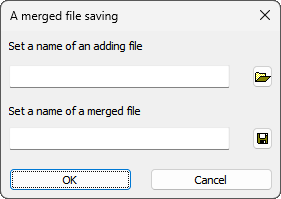
In the Specify the name of the file to be added field you must specify the name of the file whose content will be appended to the end of the current opened file. Of course, only files of the same type can be combined. In the Specify the name of the combined file field, specify the path and name of the new merged file. The file name [open file name] _add with the extension of the corresponding type is automatically offered. The OK button starts the process of creating a new combined file.
The module Mirage-L is a postprocessor of POLIGONSOFT. The program is designed to visualize the curves (graphs) prepared in the Mirage module (for more details, see the section "Drawing the curves").
You can start the module from the POLIGONSOFT shell with the Mirage-L button or from the menu Postprocessor → Mirage-L (see the figure below) or directly from the Mirage module with the View the graph files command or the button  on the panel of the working commands.
Most of the window is occupied by a field on which, in fact, the graphs are displayed (see the figure below).
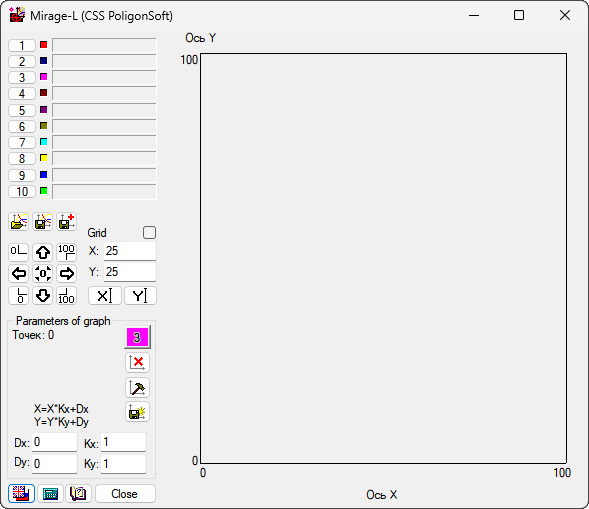
To the left of the field for visualization of the graphs are the elements for uploading the files and setting the visualization parameters (see the figure below).
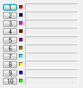
Ten identical buttons numbered from 1 to 10 located in the upper left corner of the window are used for loading the graphs files. To the right of each button there is a color indicator showing what color will be used to draw this or that graph on the coordinate field. More to the right there are the windows, in which there will be shown the full path to the files after their downloading.
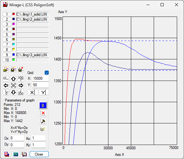
To download a file, click on one of the download buttons. A standard window of Windows applications will be opened for downloading the files. The graphics files have a LIN extension. After downloading the selected file (s), a full path to the file appears near the button, and the graph of the corresponding color appears on the coordinate field. It should be noted that by default the curve fits optimally into the coordinate field. Below, the figure shows the result of downloading several files.
Using the download buttons in turn, you can simultaneously download 10 graphs files. Be careful: every new graph, added working window, has its own digitization. The program does not reflect on the physical meaning of the graphics, but conscientiously leads them to digitize to single axes. Therefore, if the first one suddenly moved somewhere into the corner and / or compressed to small sizes when loading the next graph, this is the result of a large difference in the scales of the loaded curves.
When you click on the download button of the already downloaded file, the program will open a dialog box with two commands (see the figure below):
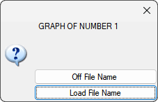
Closing the dialog with the close button in the upper right corner or pressing the Esc key leaves the situation unchanged.
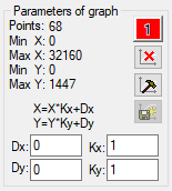
Simultaneously with the load of the file, a brief information about the graph will be displayed in the lower-left corner of the window, in the Graph parameters area: the number of the points on it, and the minimum and maximum values of the argument and function (see the figure below).
 |
The Assign the active graph button is located to the right of the graphs data. It has the color and number of the current graph. Each press on this button activates the graph with the next sequence number (after the graph number 10 again, there is a graph number 1). The information in the Graph Settings group always refers to the active graph. |
To make any graph active, without scrolling through all graphs with the help of the indicator button, you can click directly on the file name in the upper left part of the window, where the names of the graph files are displayed.
 |
The Delete the active graph butto nunloads (removes from the working field) the active graph. In this case, the file with the graph will be deleted from the list of the loaded graphs. |
 |
You can adjust the appearance of the active graph using the panel called by the Parameters of the active graph button (see the figure below). |
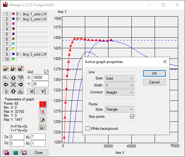
For each curve, you can customize the appearance and the thickness of the line, the type of marker and other parameters.
 |
The Create New Graph (formula) button starts the algorithm for constructing a new graph according to the formula given by the user. The button becomes active after clicking on any unoccupied position in the graphs list. After clicking on the button, you must specify the name and location of the LIN file for the new dependency. Then the Calculate graph by formula dialog opens (see the figure below). |
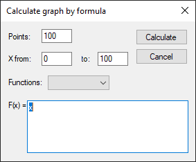
In the Calculate graph by formula dialog, you must specify the number of the points to be simulated by the given formula (function), the range of the argument (the X axis), and write the required function in the field F(x). The form of the function can be quite complicated. Above the field there is a drop-down list of the Functions containing the mathematical functions that can be used in the function (the square root, the power function, natural and decimal logarithms, etc.). The ready functions can be combined in any order. To build the function, you need to click the Calculate button.
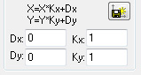
In the block Parameters of graph it is also possible to modify the active graph. You can change the K scale and set the D graph offset for each of the axes (see the figure below). To do this, just enter the required values from the keyboard into the input fields Kx, Ky, Dx and Dy. The meaning of the parameters K and D is explained by the formulas located above the input fields. After entering the parameters, the changes will be applied to the curve on the coordinate field.
When loading several curves, or when scaling and moving, it may happen that the entire graph will no longer fit on the coordinate field. In this case, there are the additional possibilities for adjusting the coordinate field. The elements that provide these capabilities are concentrated to the left in the middle part of the window (see the figure below).
 |
Four buttons with multidirectional arrows allow you to move the graph in the coordinate field window, and as the graph moves in one direction or another, the digitizing of the coordinate axes changes. The central button of this block optimally puts the graph into the coordinate field. |
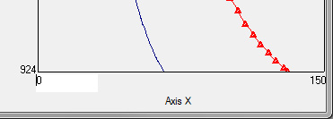
The location of the graph on the coordinate field can be affected by setting the minimum and maximum values of the argument and function along the axes of the coordinate field. To do this, use the corner buttons of the block. Clicking on each of them "highlights" the corresponding minimum or maximum value on the axis on the coordinate field and places the cursor in the input field (see the figure below). A similar result can be achieved simply by clicking the left mouse button on the corresponding value directly on the coordinate field. Next, you just need to enter a new abscissa value or ordinates at this point of the axis and confirm it by pressing the Enter key or by clicking the left mouse button on another number. The type of the graph is aligned with the new digitization of the axes.
 |
For added convenience, you can plot a mesh on the graph field. To do this, tick the Mesh box (see the figure below). The X and Y input fields below allow you to control the frequency of the mesh lines on both axes. |
 |
You can make the explanatory inscriptions for the axes of the coordinate field by pressing the X and Y buttons. Clicking on each of them "highlights" the axes signatures and places the cursor in the corresponding input field (see the figure below). |
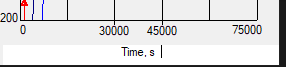
A similar result can be achieved by clicking the left mouse button on the corresponding place. Then you just need to enter the required text and to confirm its input by pressing the Enter key or by clicking the left mouse button on other fields of the same type.
The buttons in the middle part of the left field realize a number of additional features related to the saving and the use of various settings applied to the files of graphs.
 |
The Save the file with graph list button saves the status of the Mirage-L module: the loaded graphics and all view settings with a file with the CLC format. |
 |
The Read the file with the graphs list button loads the previously saved configuration file with the CLC extension, i.e. restores a certain fixed state of the module. In this case, if the previously loaded graphics files changed the contents (for example, new curves were written in them), the updated files will be downloaded. |
 |
In addition to the fact that you can save and subsequently use the files with the saved complete setting of the working window with the graphs, you can also save the actual graphics file (*.LIN) summarizing all loaded graphics into one. This can be done by clicking on the Combine the graphics and save to a file button. This file will contain all points of all loaded graphs, taking into account their modification (if any) by the specified movements Dx, Dy and the scaling factors Kx and Ky. |
It is convenient to explain the work of the last option by an example.
Suppose that two files with graphs are loaded into the Mirage-L module and for one of them the movements Dx and Dy are set so that it is an extension of the other.
You can remember these settings for two loaded graphs, as described above ("Save the file with a graphs list" button). However, suppose that you want to use these two artificially combined graphics as a single graph, which will then be loaded along with the other graphs lists that have their own settings. To do this, you can save these two graphs as one, using the "Combine the graphics and save to a file" button. In this case, a standard dialog will be called for assigning the name of the new file and its location on the disk. After saving under the specified name, you can load a new graph, like any other.


.svg)
.svg)
.svg)

.svg)