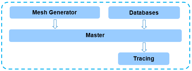
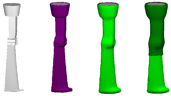
Module Master is the preprocessor of POLIGONSOFT designated for setup of three-dimensional models (GM) for simulations in the processor modules (solvers) Euler, Fourier, Hooke etc.
Preparation to the simulation consists of:
All these actions are performed in the modules of POLIGONSOFT unified in the preprocessors group.
This chapter describes the process of simulation preparation depending on the case. The Preparing the Modeling Area section describes the general principles of GM preparation, the possibilities of Master module are discussed in details. Calculation of temperature fields in a casting and a mold is the main task of modeling, regardless of the casting technology and the formulation of the problem. Therefore, the steps described in this section are required to prepare any calculation. The next sections describes how to set-up the cases of filling, radiation heat transfer, simulation of the shrinkage porosity and stress.
Next there is the description of the irregular modelling tasks, such as: exothermic sleeves, virtual mold and simulation with the non-coincident meshes and the description of the task settings of the simulation of a special casting technologies (centrifugal casting, high pressure die casting (HPDC), continuous casting and so on).
At the end of the chapter, there is the detailed description of the work with POLIGONSOFT databases.
To start the calculation, the user should perform the following actions in the Master module:
The module starts from the main window with the Master button, or the same command from menu Preprocessor.
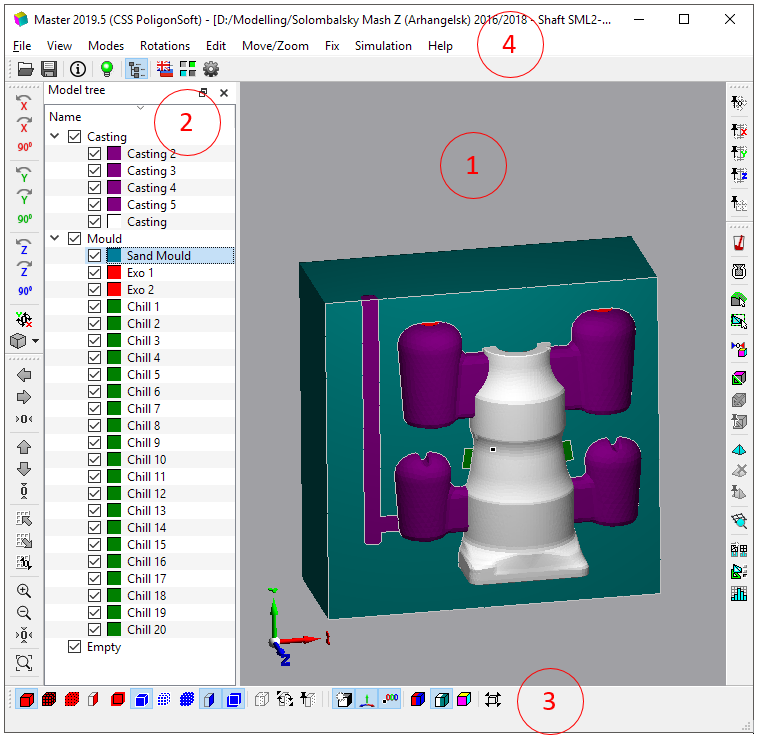
The main part of the module window (see the figure below) is occupied by the working area, where the GM is displayed (1). On the left is the Model Tree (2), which displays a list of GM volumes. The Model Tree allows you to control the visualization of the GM and set the most important parameters of the computational domain. Toolbars (3) are installed on all sides of the module window. The menu bar (4) is also installed at the top of the window.
When working with the program, you can use both the commands of the main menu in the upper part of the window, and the buttons on the toolbars. Almost all items of the main menu are duplicated by the corresponding buttons on the toolbars. Further, when describing the functions of the module, their call will be indicated only using the buttons on the toolbars, implying that there are corresponding menu items, as well as hotkeys (for some commands) indicated in the names of menu items and button tips.
The main task of module Master is to provide to the user the possibility to designate the groups of the finite elements with the different properties and their faces with different characteristics. Such identification of the faces and elements is the base of simulation process.
VOLUMES. When importing a finite element mesh of the computational domain, the Master module groups the finite elements of the mesh into volumes. The division of the computational domain into volumes (often called bodies) is usually already indicated in the imported mesh and, as a rule, is a consequence of dividing the original CAD model into volumes (i.e., even before dividing it into finite elements). The finite elements (and their faces) combined into volumes are automatically assigned some indices and types. When importing a mesh, the assignment of indices and types to finite elements will be done automatically, but often not in the way required for a particular task. Therefore, one of the user's tasks is to change the automatically specified parameters to those that correspond to the modeling task. It is also possible to create new volumes while editing the mesh. For more information on creating new volumes, see the Editing Element Indices in the Arbitrary Areas section.
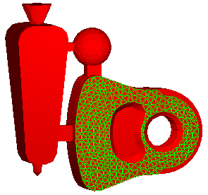
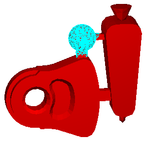
VOLUME TYPES. The finite elements included in the casting meshes have special properties and are elements of the Casting type, while the finite elements included in the mold meshes have other properties and are of the Mold type. This division is due to the fact that in addition to calculating the temperature fields, which is performed in all volumes of the calculation area, additional problems are solved in the Casting type volumes: melt flow, phase transition (solidification), formation of shrinkage cavities, macro- and microporosity, structure, etc.
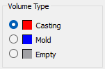
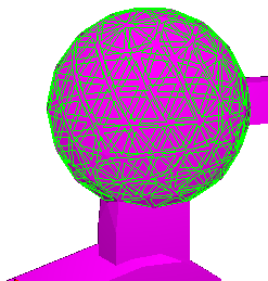
When visualizing volume types, red is used for casting bodies, and blue for the mold (see the figure below). In addition, another type can be used in the Master module - Empty. This type is used as a buffer for elements that you want to temporarily exclude from the calculation area. Volumes of this type are not visualized, but gray is used for color indexing of the Empty type in the dialog boxes of the Master module. When saving a geometric model file, all elements of the Empty type are deleted.
When importing a finite element model into the Master module, the first volume recorded in the file receives the Casting type, all other volumes - the Mold type. How to change volume types is described in the Editing Volume Types and Indices section.
VOLUME INDICES. In addition, both the casting and the mold can be non-uniform, i.e. not all finite elements entering into them necessarily have the same properties. Thus, several materials can be used simultaneously in the molds; they can have the cores, cooling plates, etc in their composition. In it’s turn the casting being monolithic and homogeneous by the physical properties, may have the areas within itself that are distinguished, for example, by the value of the initial temperature. In order to take these differences into account in the calculation, elements with the same conditions or properties are combined into groups and assigned numbers or indices.
There are 9 element indices in total, and they are numbered from 1 to 9. To visualize volumes consisting of elements with different indices, POLIGONSOFT uses a specific color scheme (see the figure below).
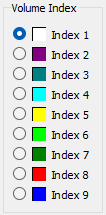
The element index (and its color) means that some condition or property (physical parameters, temperature, etc.) will be assigned to this group of elements. These conditions and properties must also be defined in the Master module by connecting the appropriate databases, templates and process conditions. For example, for volumes of the "mold" type, the index of the element always determines the its material. The properties of this material will be assigned to this volume when connected mold material properties to the model. At this stage, it is advisable to connect one of the technological process templates to the Master module in order to view ready-made sets of mold materials and determine volume indices. This is done in the Start Simulation and Parameters window on the General tab in the Mold Properties line or on the Project Overview tab in Master module window.
Accordingly, if the same properties or conditions are assigned to elements with different indices, then these elements will behave in the same way during simulation. Such an indexing system makes it possible to economically and efficiently set a wide variety of simulation conditions, for example, two domains of identical materials can easily be assigned the same thermophysical properties, but different initial temperatures.
When the model is first loaded into the Master module, the volumes are consecutively numbered, i.e. the first volume gets index 1, the second one gets index 2, and so on. If there are more than 9 volumes in the model, the tenth volume will again receive index 1, and so on. How to assign the element indices is described in the section on editing the indices of volumes and arbitrary areas.
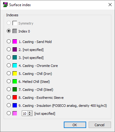
BOUNDARY INDICES. The faces of finite elements can be in different conditions: one thing is the face of an element that is on the boundary between the casting and the mold, and quite another thing is the face of an element that is on the outer boundary of the casting, i.e. between the casting and the environment. For this reason, the faces of elements that form boundaries (surfaces) with certain conditions are assigned the same index. Each specified boundary index reflects the processes that occur during the transition from one volume of the computational domain to another (most often, this is heat transfer, for example, from the casting to the mold). Indices are assigned only to the outer faces of the elements of the volumes of the Casting and Mold types, i.e. the Casting-Mold, Casting-Environment and Mold-Environment boundaries. The faces of elements that are in contact with faces of the same type (i.e. Casting-Casting and Mold-Mold) may not be specially indexed, since at the boundary of their contact, no jump of the modeled function (for example, temperature distribution) is assumed and, therefore, there is no need to specify the characteristics of the process of transition through such edges. Such edges are automatically assigned the index 0, they are not available for assigning a boundary index. How to assign boundary indices is described in the section on editing the boundary indices.
There are 19 boundary indices in total, and they are numbered from 0 to 18. POLIGONSOFT has some rules for assigning boundary indices that cannot be violated. In particular, zero indices are assigned to symmetry boundaries, internal boundaries, and surfaces with zero flows (from the point of view of thermal, diffusion, filtration, electrical, etc. flows, all these are boundaries of the same type).
Indices from 1 to 9 can be assigned to both external boundaries and boundaries between volumes (e.g., between a casting and a mold). In this case, even if there is actually nothing beyond such a boundary, solvers will assume that some conventional “semi-infinite” mold is implied behind this boundary. The material properties of such a virtual mold will be used in accordance with the index that this boundary has. This rule is valid for both casting boundaries and mold boundaries – in any case, the virtual volume will be considered a Mold. The problem of modeling with a virtual mold is described in more detail in the Virtual Mold section. This indices also can be assigned to the boundaries between the casting and the ambient with assigned temperature.
Indexes from 10 to 18 can be assigned only to boundaries with the environment. However, if there is actually a body behind such a boundary, the solvers will still consider it to be a boundary with the environment (this can be used if for some reason it is necessary to "disable" the connection between the casting and the mold in the calculation).
Just like for element indices, boundary indices correspond to some physical parameters, for example, heat transfer parameters. They are assigned when connecting one of the process templates in the Start Simulation and Parameters window on the General tab in the Heat Transfer Parameters line. Just like for element indices, a certain color scheme is adopted for edges, used when visualizing boundaries (see the figure below).
It should be noted that at the boundary between two elements of different types there are always two faces – the face of one element and the face of the other element (see the figure below).
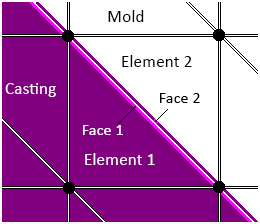
In general, each of these faces can have its own index, for which unique conditions can be set. But in normal conditions, when modeling casting technologies, the same parameters are set for both faces. Therefore, either such faces have the same boundary index, or they have different indexes, but the parameters assigned to these indices are similar.
When a mesh model is first loaded into the Master module, all faces are assigned default indices: the Casting-Mold boundaries are assigned index 1 on the casting side and on the mold side. The Casting-Environment boundaries are assigned index 17, and the Mold-Environment boundaries are assigned index 18. If one of the process templates is connected to the Master module, the user can see which parameters are assigned to each boundary index. The template is connected in the Start Simulation and Parameters window on the General tab in the Heat Transfer Parameters line. The template is configured in such a way that when using the default boundary indices, the user in most cases receives a fully configured heat transfer model for the selected process.
If necessary, you can change the boundary indices to create additional conditions on the boundaries. For example, some of the outer boundaries that are considered "by default" as boundaries with the environment may actually be symmetry boundaries and should be assigned the index 0.
When first loaded, the first volume of the mesh model is assigned the Casting type, and all other volumes are assigned the Mold type. This is often not the case, and the user assigns volume types independently. After editing volume types, you will need to reassign the default boundary indices (for more information, see the Editing Boundary Indices section).
This section provides a complete listing of toolbars commands . As mentioned above, almost all the menu items are duplicated by the corresponding buttons on the toolbars. Each command is given a short description and a link to the corresponding section.
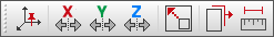
The most common functions (loading GM, recording GM, etc.) are concentrated on the Standard toolbar in the upper part of the preprocessor window (see the figure below)

 |
The Open Geometry (Ctrl+O) button is used to load the mesh model in different formats. See Loading and saving the model section for more details. |
 |
The Save Geometry (Ctrl+S) button saves the geometric model with all the assigned conditions and calculation parameters in the POLIGONSOFT format with the g3d extension. See Loading and saving the model section for more details. |
 |
The Model Information (Ctrl+I) button opens a window that contains information about the loaded geometric model. See Model Information section for more details. |
 |
The Start Simulation and Parameters (Ctrl+R) button opens a window where all the required simulation data is set and the calculation starts. See Simulation chapter for more details. |
 |
The View Results button launches the postprocessor to view the calculation results. See Viewing Results chapter for more details. |
 |
The Model Tree button enables displaying the model tree on the left side of the Master module window. For information on using the model tree, see Editing Volume Types and Indices section. |
 |
The Language (F3) button cyclically changes the interface language. Press it several times to switch to the desired language. |
 |
The Special Colors button opens the Master module settings window, where you can set the background color of the workspace, casting mesh, mold mesh, section plane color, border and element mark colors. See Special Colors. section for more details. |
 |
The Settings (Ctrl+Alt+S) button opens a window that contains all the parameters that control the preprocessor work and its individual functions. See Module Settings section for more details. |
Functions and tools associated with the case setup (materials, process parameters, boundary and initial conditions) are called by buttons:
 |
The Material Properties button opens the editor where the materials used in the calculation are created and edited. See Material Properties section for more details. |
 |
The Inlets button opens a dialog where you can specify the locations of the melt inlets into the mold, their sizes and parameters. See Melt Inlet section for more details. |
 |
The Heat Transfer button opens the editor where heat transfer parameters are created and edited at the boundaries between volumes (body-body) and at external boundaries (body-environment). See Heat Transfer Parameters section for more details. |
 |
The Temperature Modes button opens the editor where the temperature modes of the casting and mold volumes are created and edited. See Temperature Modes section for more details. |
 |
The Rotation button opens a dialog where you can set the speed and direction of rotation of the model during centrifugal casting. See Centrifugal Casting section for more details. |
 |
The Translation button opens an editor where modes for moving casting and mold volumes are created and edited. See the Translation Modes section for more details. |
 |
The Dynamic Environment оbutton opens an editor where you can create and edit an environment consisting of several layers with different parameters. See the Dynamic Environment section for more details. |
 |
The Nucleation button opens an editor where the parameters for the nucleation of the grain structure at the casting boundaries are created and edited. See the Surface Nucleation section for more details. |
 |
The Inheritance button opens an editor where the macrostructure inheritance parameters at the boundaries of the calculation area are created and edited. See the Structure Inheritance section for more details. |
The largest number of special functions of the Master module are called by the buttons on the Edit toolbar, which by default is located along the right border of the Master module window.

 |
The Create Shell button opens a dialog for creating a shell of a given thickness around the selected bodies. See Shells Creation section for more details. |
 |
The Extrude Mesh button opens a dialog for creating new volumes by extruding a surface mesh at a specified distance. See New Volumes Creation (Extrude Mesh) section for more details. |
 |
The Select Contiguous button turns on the surface selection mode. See Editing Boundary Indices section for more details. |
 |
The Select Elements by Frame button turns on the frame selection mode. See Editing the indices of the elements in the arbitrary areas section for more details. |
 |
The Set Default Boundary Indices button assigns default boundaries for the entire GM. See Editing Boundary Indices section for more details. |
 |
The Select Boundaries button opens a dialog for selecting boundaries by index. See Editing Boundary Indices section for more details. |
 |
The Deselect All Boundaries (Ctrl+G) button deselects all the selected boundaries. See Editing Boundary Indices section for more details. |
 |
The Assign Boundary Index button opens a dialog for assigning an index to the selected boundaries. See Editing Boundary Indices section for more details. |
 |
The Select Elements button opens a dialog for selecting elements by index. See Editing the indices of the elements in the arbitrary areas section for more details. |
 |
The Deselect All Elements (Ctrl+E) button deselects all selected elements. See Editing the indices of the elements in the arbitrary areas section for more details. |
 |
The Assign Volume Index button opens a dialog for assigning an index to the selected elements. See Editing the indices of the elements in the arbitrary areas section for more details. |
 |
The Check Mesh Quality button checks the mesh quality according to various criteria and opens a dialog for viewing the report and correcting bad elements. See Mesh Quality Control section for more details. |
 |
The Refine Mesh button performs a shift of mesh nodes to improve its quality. See Mesh Quality Control section for more details. |
 |
The Split Elements button opens a dialog for choosing an algorithm for remeshing the selected mesh fragment. See Mesh Quality Control section for more details. |
 |
The Mark Parameters button opens the preprocessor settings window for selecting parameters and display styles for selected elements and boundaries. See Mark Parameters section for more details. |
 |
The Mesh Quality button shows a histogram of the deviation of mesh elements from an ideal tetrahedron. See Mesh Quality Control section for more details. |
Commands changing the geometric model: its orientation, shape, size, position, etc., are located on the Transformation toolbar (see the figure below).
 |
The Fix Rotation button rotates the coordinate system to its base position (front view), and changes the orientation of the model in space. |
 |
The Reflect by X button flips the geometry around the X axis. |
 |
The Reflect by Y button flips the geometry around the Y axis. |
 |
The Reflect by Z button flips the geometry around the Z axis. |
 |
The Scale button resizes the model. |
 |
The Copy/Move button copies or moves the visible bodies of the model in the given direction. |
 |
The Measure (F4) button opens a tool for measuring the distance between two given points. |
For more details about each command, see the Change Model Orientation, Position and Size section.
|
Settings button on the Standard toolbar opens a window that contains all the parameters that control the work of the preprocessor as a whole and its individual functions. To open the settings window, you can use the key combination Ctrl + Alt + S (see the figure below). |
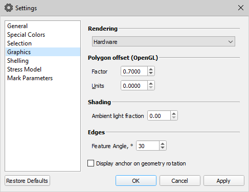
The settings are grouped in tabs, according to the list on the left side of the window. To take effect, you should click the Apply button. However, as a rule, these settings do not require constant adjustment. The default values set the maximum comfort when working with the geometric model. The models settings and settings for some special functions specified in this window will be described further in the corresponding sections. This section describes settings that affect the preprocessor operation.
To return to the default module settings, click the Restore Defaults button in the lower left corner of the window and then confirm the selection with the OK button. The settings for the active tab are reset. Selecting Reset All resets all module settings.
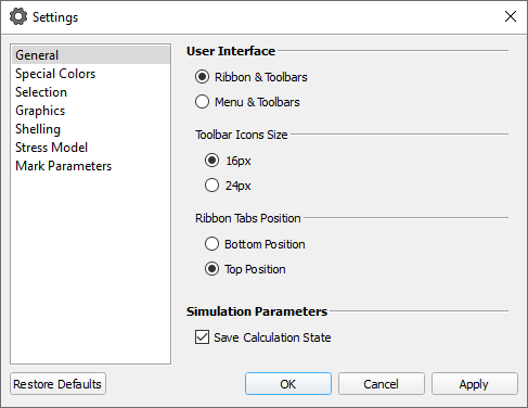
The General tab contains user interface settings (see the figure below).
Sets the general appearance of the user interface - tabbed ribbon menu or classic menu. In both cases, you can additionally use toolbars. Default value: Ribbon and Toolbars.
|
The Special Colors button on the Standard toolbar opens the Settings window on the corresponding tab where the user can set the background color, casting mesh color, mold mesh color, section plane color, edges and element label colors (see the figure below). |
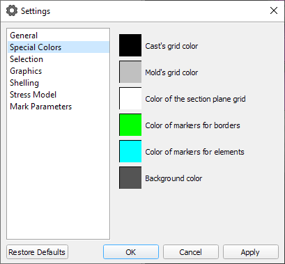
To set a color, click on the corresponding colored square. The standard MS Windows Color Picker window will open. Having set the desired color in it, you should click OK button to return to the window for setting Special Colors. After making all the changes, click the OK button.
The section plane color has a checkbox Auto (it is checked by default). This means that when setting up the section plane, its color will be automatically set to black or white depending on the set background color of the window. If the checkbox is disabled, the color specified by the user will be used.
The visualization of the selected (marked) elements or their external faces is performed using marks - highlighting the edges of the faces and / or a point in the center with color (see the figure below).
|
The style of marks can be changed by the user. To do this, you can use the Selection Settings button on the Edit toolbar or the Settings tab of the ribbon menu. The Settings window will open, where the Selection tab contains the settings that determine the appearance of the element and face marks (see the figure below). |
 |
 |
Boundary selection result |
Element selection result |
|
The color of element and face marks is set in the Settings window, which can be opened by pressing the Special Colors button on the Standard panel (for more details, see the Special Colors section). |
At the top of the tab there is an option Select boundaries together with opposite. If the option is enabled, then when selecting internal mated boundaries of the "cast-mold" or "mold-to-mold" type, a new boundary index is assigned simultaneously to both of its sides. For example, if you assign a new index to a casting-chill boundary on the chill side, the casting-side boundary will automatically get the same index. When this option is off, you can assign different indexes to mating boundaries. Option is enabled by default.
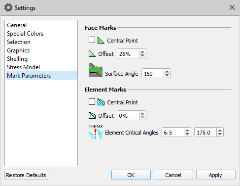
Below are two groups of parameters: Face Marks and Element Marks. With their help, you can achieve the most convenient marks visualization.
  |
Central Point options draw a point at the center of the marked triangle or element. The parameter is disabled by default. |
  |
The Offset options control the visual gap between selected objects. When the gap is zero, the edges of the object are painted directly, and when the gap is increased, the edges of the marks are drawn inside the selected object. Specified as a percentage. |
 |
The Surface Angle parameter specifies the criterion for determining whether adjacent feature faces belong to the same surface. If the dihedral angle between adjacent faces is equal to or greater than the specified value, the faces are considered to be on the same surface. This allows you to select faces not element-by-element, but immediately with surfaces. For example, if you set the parameter equal to 180°, the faces that lie in the same plane will be selected, and if the parameter value is 0°, all the edges of the object are selected. The parameter is set in degrees from 0 to 180. The default value is 150°. |
 |
The Element Critical Angles parameter specifies the minimum and maximum dihedral angles in degrees. These values are used when analyzing the finite element model for quality. The default limit angles are set to 6.5° and 175°, which usually do not need to be changed. For more information on checking the mesh quality, see Mesh Quality Control section. |
The creation of three-dimensional geometric model and its dividing to the finite elements are the complex processes requiring the specialized software. The programs performing the dividing operation save the results of its work in the original file formats. That’s why all models prepared in the external mesh generators should be converted from their formats to the internal format of POLIGONSOFT.
Initially, the working field of the program is free, and most of the buttons on the toolbars are unavailable. And this is natural, since the source file containing the geometric model (GM) has not yet been loaded into the program. Recall that from the point of view of numerical simulations by the finite element method, the geometric model is a finite element mesh.
|
In order to load the GM, you should click the Open Geometry, button, usually located in the upper left corner of the window on the Working commands toolbar. You can also use the drop-down menu of the "File" menu item or the Ctrl+O key combination. |
Note that the menu items duplicate all buttons on the toolbars. In the description we will go from the buttons of the toolbars, without mentioning each time about the presence of a similar item in the submenu and the hot keys noted there.
After clicking the Open Geometry File button, the Loading Options window will open.
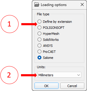
In this window, use the radio buttons to select the file type (1) that you want to download. The possible file types cover formats of almost all modern programs intended for dividing the geometric models into the finite elements: FEMAP, HyperMesh, NASTRAN, PATRAN, ANSYS, CADDS, NX, CATIA, ProCAST and SALOME (supplied with POLIGONSOFT). Selecting the POLIGONSOFT type means that it will load a file that has already been saved in POLIGONSOFT format.
Then you can specify the units in which the coordinates of the nodes in the downloaded file (2) are recorded or specify the unique scale factor. In various CAD-systems and mesh-generator programs, the coordinates of points of the geometric objects are specified in different units of length: millimeters, inches, meters, etc. POLIGONSOFT relies on the SI system, and measures all coordinates in meters. Therefore, in order to observe the true size of the geometric model, the corresponding coordinate resimulation should be performed. For example, in the transition from millimeters to meters, all coordinates should be multiplied by 0.001. To change the current scale factor, you should normally set the text cursor in the input field and enter the corresponding number on the keyboard. To check how the program responded to the introduction of the scale factor, you can check the size of the model on the Information Panel. (It is called by a special button, which will be described below.)
After clicking the OK button, Open Geometry File window will open, in which you can find the file to be loaded on the disks.
If you select the Define by Extension radio button in the Loading Options window, it will be possible to load any file with a finite element mesh, since the filter All files (*. *) will be used. When loading, the units of length previously set for the selected file type will be used. If you try to download a file that does not match any of the used formats, an error message will be displayed.
Files can also be loaded by dragging them onto the working area of the preprocessor window.
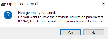
In POLIGONSOFT there is a possibility of inheriting the parameters specified during the preparation of the previous simulation. This is very convenient when you need to simulate the same casting, but with a different gating-feeding system under the same (or close to the same) conditions. In such cases, most of the parameters such as: casting alloy, mold materials, heat transfer parameters, initial temperatures, etc. remain unchanged and can be translated to a new geometric model. Therefore, after loading the mesh, a message is displayed (see the figure below), in which it is proposed to apply the parameters of the previous calculation to the loaded geometry (Yes button), or load the default calculation parameters (No button).
After loading the model, an image of the modeled object will appear in the workspace, and most toolbar buttons will become active. By default, the geometric model is displayed in casting and mold surface mode, or as configured by the user during the previous preprocessor run. Managing geometric model visualization is discussed in the Common Elements of 3D Modules chapter.
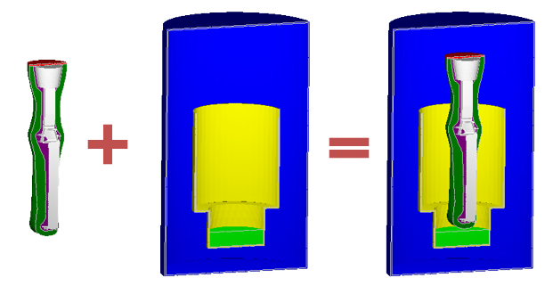
In the preprocessor Master it is possible to add other GM from previously created geometry files to the loaded model. This can be convenient if some of the GM bodies involved in the calculation do not change in the process of technology development. For example, when simulating vacuum casting, a furnace with heaters is involved in the calculation. This GM can be added to any model of the casting block that is planned to be filled in this furnace (see figure below). Of course, both GMs must be performed in a single coordinate system. To add a GM, select the Append Geometry ... command from the File menu and load the required file.
A list of previously opened geometry files is stored in the File-Recently Open Files menu.
|
The Save Geometry command will save the geometric model with all the assigned conditions and calculation parameters in the POLIGONSOFT file with the g3d extension, in which it is ready for calculation. To call the command, you can use the key combination Ctrl+S. |
After clicking the Save Geometry button, a standard dialog will open, in which you can specify a file name and specify its location on disk. By default, in the Save Geometry dialog, in the File Type field, the "Geometry Files (* .g3d)" filter is set. When saving with this filter, a geometry file will be saved in the specified location and a DATA folder will be created, into which files with additional data necessary to start the simulation will be written. If you need to run the calculation on another computer or in a different folder, copy the g3d file and the DATA folder to a new location, open the geometry file in the Master module and all the simulation parameters will be updated.
It is also possible to save the geometry file without additional data, i.e. only a finite element model without reference to the given simulation parameters. To do this, in the save dialog, change the file type to "Mesh only (* .g3d)". In this case, only the g3d file will be saved, no DATA folder will be created.
In POLIGONSOFT, the gravity vector is always directed against the Y-axis and this is important for the correct calculation of shrinkage porosity. This is not always taken into account when creating a CAD model of a casting and a mold, therefore, after loading the mesh model into the Master module, it may be necessary to change its orientation. In this case, it is necessary to fix the visual angle of rotation, i.e. enter it into the real coordinates of the GM. The corresponding commands are located on the Transformation Toolbar.
Remember that when you rotate the object (s) in the working area (see the Common Elements of 3D Modules section), the view or the viewing angle of the model changes, but the orientation in the coordinate system remains the same, because the coordinate system rotates with the object.
 |
Click the Reset Rotations button on the Rotations toolbar to set the model to a base position: the X-axis is horizontal, the Y-axis is vertical, and the Z-axis is perpendicular to the plane of the screen. This position corresponds to the front view. |
In the base position, it is clear how the model is oriented in the POLIGONSOFT coordinate system. For example, on Fig. below (left) you can see that the loaded model is oriented incorrectly. For convenience, you can turn off the display of form volumes in the model tree. Use the buttons on the Rotations toolbar to set the correct position of the model. For example, for the case shown in Fig. below (left), you need to double-click the Rotate Across X 90° button to rotate the model 180° around the X axis.
Do not use the mouse to rotate the model! Adjusting the exact position with the mouse "by eye" is not possible. Use the buttons on the Rotations toolbar.
|
After the model is in the correct position on the screen, click the Fix Rotation button on the Transformation toolbar. |
When you click on the Fix Rotation button, the position of the object in the working area will remain unchanged, but the coordinates of the mesh nodes will be recalculated, and the coordinate system will unfold to the base "front view" position (see the figure below on the right). Now the direction of the gravity vector (against the Y-axis) corresponds to the technological process.
|
|
Front view before rotation |
Front view after rotation |
In some cases, additional editing of the model may be required, for example, its scaling or mirroring about one of the axes.
In some cases, it is necessary to mirror the geometric model along an axis. This means that the coordinates of all points along this axis will be reversed. To do this, use a group of three buttons on the Transformation toolbar.
|
The Reflect by X command flips the geometry around the X axis. |
|
The Reflect by Y command flips the geometry around the Y axis. |
|
The Reflect by Z command flips the geometry around the Z axis. |
Press the desired button to get the result. If the wrong button was selected by mistake, you must press it again to return the model to its original position. In Fig. below is the result of flipping the model along the Y axis.
|
|
Before reflection |
After reflection |
Sometimes you need to change the dimensions of the model. Most often, such a need arises if the units of measurement were specified incorrectly when importing the mesh (for more information, see the Loading and saving the model section).For the dimensions of a model, see the Model Information section.
|
The Scale button on the Transformation toolbar opens a dialog where you can set the scaling factor of the model (see the figure below). |
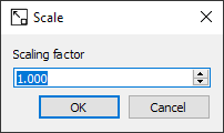
Enter the desired value in the Scaling factor field and click the OK button. You can control the result in the Model Information window.
You can create copies of one or more model volumes or move these volumes in a given direction. This can be useful, for example, when modeling the filling of several identical molds standing side by side. In this case, there is no need to create mesh models for all molds.
|
The Copy/Move button on the Transformations toolbar opens a dialog where you can set the direction of copying or moving the visible volumes of the model (see figure below). |
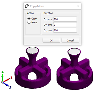
In the left part of the dialog, select the action to be performed. In the right part of the dialog, you need to enter the components of the displacement vector in mm. Clicking the OK button will complete the operation.
Note that the action is performed only for visible objects (visibility is set in the model tree). It should be noted that the intersection of grids is not allowed.
|
The Measure (F4) button opens a tool for measuring the distance between two given points (see figure below). |
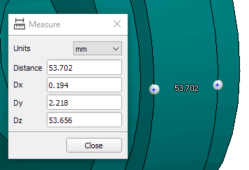
To put a point, you need to right-click while holding down the Ctrl key. After two points are set, the distance between them is shown in the drawing area. The dialog displays the length of the segment between two points and the length of its projections on the coordinate axes.
To remove a point, you need to click the left mouse button while holding down the Ctrl key.
 |
Use the Reset button (Ctrl+D) to remove all points and reset the dialog state. |
At the beginning of the loaded model set-up for calculation, it is advisable to load all the necessary materials into the project: casting material and mold materials. This can be done in the Start Simulation and Parameters window on the General tab by filling in the lines Alloy Properties and Mold Properties (see the figure below).
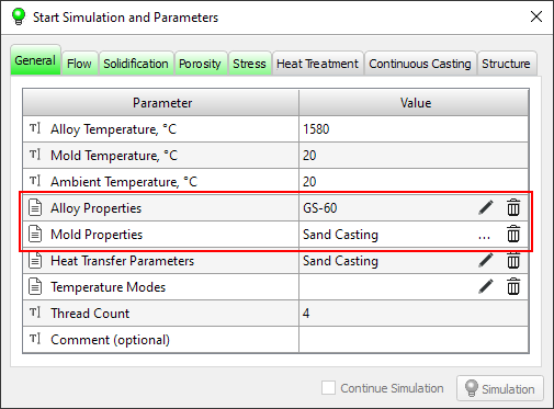
At the end of each line there are icons for necessary operations are performed.
 |
The button is located in the Mold Properties line and loads files of the pmms type (or the obsolete bdf type) into the project, which can contain up to 9 mold materials used for a particular casting technology. Such files can be loaded from the POLIGONSOFT database and edited by the user (see later in this section). |
 |
The button is located in the "Alloy properties" line and opens the material editor, where the user can load the material from the POLIGONSOFT database or enter his own data. See the Material Properties section for details. |
 |
The button removes data from the project and clears the line. |
Another way to assign materials is the Materials tree, which is located on the Project Overview tab (1) in the Master module main window (see the figure below). To set the casting material, press button in the corresponding line (2). The material editor will open and you can import the required material from the database (see the Material Properties section for more details).
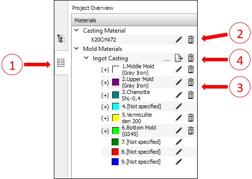
МThe mold materials can be specified in the same way as the casting material, i.e. importing each material for each mold volume index directly from the material database. To do this, successively press buttons opposite each desired volume index (3) and load the material through the Material Properties editor. Volume indexes assigned to mold bodies are marked with a "(+)" at the beginning of the line. If desired, you can save the loaded set of mold materials to a pmms (POLIGONSOFT Mold Materials Set) file and then use it in other calculations, to do this use the  button (4). Such files, created for different cast technologies, are in the POLIGONSOFT database, and they can be loaded with a button (loading of obsolete bdf files is supported).
As described in Basic Concepts: Volumes, Types, Indexes section, in the imported mesh, finite elements are grouped in volumes according to the casting and mold design. Preparing the calculation, all volumes of the model should be assigned one of two types: "casting" or "mold". In addition, each volume is assigned a number or "index", which means that this volume is assigned some condition or property (physical parameters, temperature, etc.). These conditions and properties are set through the connection of the corresponding databases, templates and process conditions. For example, for "mold" volumes , the volume index always determines its material. The properties of this material will be assigned to the volume by the index number from the loaded mold materials property set. Below, in the table, there is a list of properties and conditions that can be assigned to the volumes of the model through the volume index. Note that this list is not the same for casting and mold volumes.
| Property / Condition | Casting | Mold |
Material Properties |
|
+ |
Temperature Mode |
+ | + |
Translation |
+ | + |
Separation of the volume mesh |
+ | + |
Filled volume |
+ |
|
Radiation Area |
+ | + |
Empty for stress |
|
+ |
Removable element of the |
+ |
|
Positions that are linked only to the volume index and do not depend on its type are highlighted in green. This means that by assigning the same volume indices to the casting and mold volumes, you can set them the same conditions, for example, the temperature mode or translation. This can have undesirable consequences, so you should carefully consider what conditions are associated with the selected index.
When importing a mesh created in a mesh generator, the first volume recorded in the file gets the "casting" type by default, all other volumes - the "mold" type. At the same time, the volumes receive continuous numbering, i.e. the first volume gets index 1, the second - 2, and so on. If there are more than 9 volumes in the model, the tenth volume will get index 1 again, and so on. In most cases, the "default" settings do not correspond to the real situation and you need to manually specify the Type and Index parameters for each model volume.
Before you start editing the types and indices of volumes, you should connect one of the templates of the technological process (for example, mold materials file) to the Master module in order to establish a connection between the indices of volumes and the materials of the mold. This is done in the Start Simulation and Parameters window on the General tab in the Mold Properties line(see details in the Сommon Simulation Parameters section). System templates for different technological processes are located in the %POLIGONSOFT%\Database folder.
|
In order to reassign indices or volume types, the model tree is used, which is displayed by clicking the Model Tree button in the Standard toolbar (button pressed by default). |
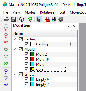
The tree contains a list of all the volumes available in the simulation area (see the figure below). The volumes are distributed in three tree branches according to the type (Casting, Mold or Empty). By default, all volumes have names according to the type to which they belong and consecutive numbering (for example, "Casting 1" "Mold 2", "Mold 3", "Empty 4").
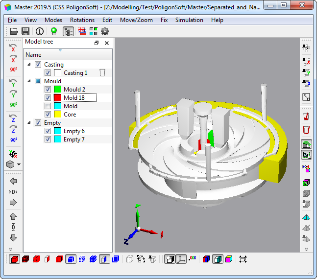
Each position in the tree has a switch that controls the visibility of the volume or the entire group of volumes. When the switch is off, the selected volume or group will not be displayed in the working area of the module. When the switch is on, a volume or a group of volumes is displayed on the workspace. The display mode is set by the buttons on the Modes panel (see details in the Model Display Modes section). The display of the volumes of the Empty group is always disabled and cannot be enabled. To display volumes from the "Empty" group, you need to change their type to Casting or Mold. Each volume in the tree has a color indicator indicating the volume index in accordance with the color scale adopted by POLIGONSOFT (for more information on the indices of elements (volumes), see the Basic concepts: Volumes, Types, Indices section).
To the right of the name are condition indicators. They become active if any conditions associated with its index are assigned to the volume. By clicking on the active indicator, you can edit the specified condition, this is described in the corresponding sections below.
Some of the commands described below are available through the context menu of the tree (see the figure below), the content of which varies depending on the mode of object selection - one at a time or a group one.
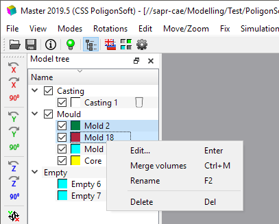
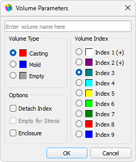
To go to volume editing, double-click with the left mouse button on its name in the model tree, or on the volume itself in the working area of the module. This will open the Volume Parameters window (see the figure below). You can change the parameters of not only each volume separately, but also a group of volumes. To do this, select the required volumes in the model tree, and then open the volume parameters window through the context menu of the model tree or by pressing the Enter on the keyboard.
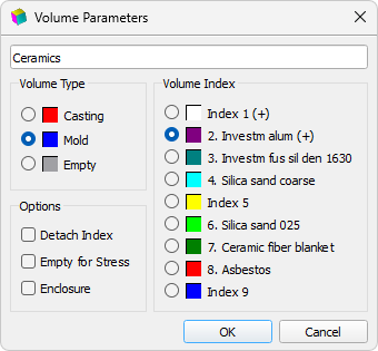
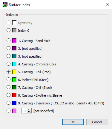
At the top left, in the Name field, the name of the edited volume is indicated, which can be changed. Three radio buttons on the left side of the window allow you to change the type of volume, and the nine radio buttons on the right - its index. The plus sign (+) to the right of the index number indicates that this index has already been assigned to some volumes of the model. This does not prevent you from applying this index again, the model may contain several volumes with the same index (for example, if they are made of the same material).
The figure above shows the view of the window for editing the volume parameters when the volume type "Mold" is selected. In this case, the volume index always specifies the volume material of the mold, so the material names are written next to the indexes. The list of materials and the correspondence of these materials to indexes are set by the user on the Project Overview tab independently by loading materials from .pmat files or by loading a process template, i.e. mold materials file .pmms (for details, see the Materials Assignment section). If the volume type is Cast or Empty, the volume index list does not contain useful information. In general, casting bodies can have any indices , because usually they are not given special conditions or special technological parameters. However, in some situations (for example, when using internal chills), the volume index of the casting can be important. This is discussed in the relevant sections.
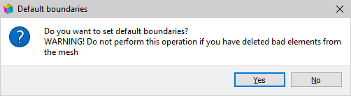
Changing the volume parameters is completed by pressing the OK button. If the volume type was changed during editing, a message will be displayed prompting you to assign default boundaries (see the figure below). This happens because after the volume type changing , the numbering of its boundaries contradicts the accepted "standard" indexing of the outer borders (by default, these are indices 17 and 18). The default numbering of boundaries is discussed in the Basic concepts: Volumes, Types, Indices section. The operation of assigning the default boundaries usually facilitates the preparation of the model, but in some cases it is undesirable (for example, when deleting "bad" elements, see the section "Mesh Quality Control" about this). If you agree to assign the default boundaries, you need to click the Yes button, otherwise, click No.
If you want to change only the type of volume or volumes (without changing their indices), you just select these volumes in the tree and drag them to the desired group.
By default, the "Master" establishes none-ideal contact at the casting-mold interface and ideal contact between the mold volumes. In other words, the casting and mold are FE mesh with coincident nodes at the contact boundary. Bodies of the "Mold" type represent a equivalent mesh, the elements of which can have different properties, depending on which index is assigned to them. You can split the meshes of mold bodies so that a mold-to-mold boundary forms between them, where you can set the heat transfer conditions (none-ideal contact). To do this, select the detachable volume in the model tree, double-click the window to edit the volume parameters, and tick the Detach Index checkbox located under the Volume Index group. After pressing the OK button, indices corresponding to the required heat transfer parameters should be assigned to the boundaries of the separated volume (the procedure for assigning these parameters is described in the Heat Transfer Parameters section). The separated volume has an interactive indicator (see the figure below), i.e. you can separate volumes directly in the model tree by clicking the mouse in the corresponding cell opposite the volume.
It should be noted that when detaching the mesh of a volume with a selected index, all volumes with the same index and type will be automatically detached (in the example under consideration, all volumes of the mold with index five (yellow) will be detached). In this case, the boundaries between the separated volumes and the remaining bodies of the mold will remain zero (they have index 0 by default). If such boundaries are not assigned new indices with the required heat transfer parameters, i.e. index 0 remains assigned to them, they will be processed by the solvers as adiabatic (condition of no heat transfer).
Casting volumes can also be detached to solve highly specialized problems. In this case, the same rules for assigning boundaries described above apply to them.
Additional volume control commands are available through the context menu of the tree:
 |
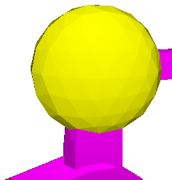
To see the results of the Type assignment, you should enable the coloring of the model by volume types by clicking the Show Volume Types button on the Modes panel. |
 |
To see the results of assigning the Element Indices, you should enable the model coloring by the volume indices by clicking the Show Volume Indices button on the Modes panel. |
More details about display modes see in the Model Display Modes section.
Sometimes it is necessary to change the model, for example, delete fragments of some volumes or assign new properties to some arbitrary area of it. Typically, this requires changes in CAD and create a new FE model in the mesh generator, but in some cases, these operations can be avoided. To do this, it is possible to create a new volume from an arbitrary group of elements and assign the necessary parameters to it: type and index, in Master module. The concepts of "type" and "index" of an element are described in the Basic concepts: Volumes, Types, Indices section.
To select elements, use a group of buttons on the Edit toolbar (see the figure below). Some of the buttons in this group may be inactive if there are no selected elements in the model.

To create a new volume within the existing model, you need to select the required group of elements and assign new parameters to it.
|
The easy way to select elements is to use Select Elements button. This opens the dialog box (see the figure below), where you can use the checkboxes and radio buttons to describe the group of elements that you want to select. |
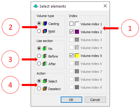
To select elements of one or more indices, you need to check the corresponding lines in the right part of the window (1). Only those volume indices that are used in the model are available for selection. The radio buttons (2) indicate where to select the elements of the selected indices - in the casting or in the mold. Depending on the selected volume type (2), the list of volume indices available for selection (1) changes. Radio buttons (3) set how to select elements, selected (1) indices and located in specified (2) volumes, in relation to the section plane. Either all elements satisfying conditions (1) and (2), or their part located before or after a given section plane can be marked. To use condition (3), you must first set the section plane to the desired position. How to control the section is described in the Section Plane section.
Finally, the radio buttons (4) set the operation on a given group of elements - select or deselect.
It should note, that an element is considered to be located on any side of the section plane if all four of its vertices are located there.
After the group of elements is set, click the OK button in the Select Elements dialog to apply the selection operation.
|
Another quicker way to select elements is to select it by frame. To activate this method, you should click Select Elements by Frame button. The button will remain pressed. |
It should be noted that the selection of elements in an arbitrary way, without relying on the types and volume indices assigned to them, can be a rather laborious procedure.
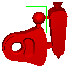
When the pressed button Select Elements by Frame, the combination Shift+LMB allows you to stretch a frame of the required size in the working area (see the figure below). All elements that are entirely within the frame area will be selected. The selection result is shown in Fig. below. This operation can be repeated several times to obtain the desired result.
 |
 |
a) |
b) |
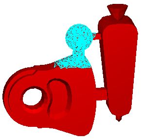
The Shift+RMB combination allows you to set an area with a frame to deselect a part or all selected elements (see the figure below). All elements that fall entirely within the frame area will be deselected. This operation can be repeated several times to obtain the desired result.
 |
 |
a) |
b) |
The appearance of the marked elements (tags) is determined by the settings (see the Mark Parameters section).
|
The selected elements can be assigned a new index and other parameters. To do this, click the Assign Volume Index button on the editing panel. The Volume Parameters dialog will open (see the figure below). |
In the Volume Parameters dialog, you can assign a name, type and index to a group of selected elements. After pressing the OK button, a new volume will appear in the model tree, and the selection will be canceled.
Other operations with volumes are described in the Editing Volume Types and Indices section.
|
All available marks can be removed by clicking the Deselect All Elements button on the Edit toolbar or using the Ctrl+E hotkeys. |
|
To see the result of assigning indices to selected elements, you can turn on the GM visualization by volume indices by clicking the Show Volume Indices button on the Modes panel. This is described in more detail in the Model Display Modes section. |
All faces of the elements of each GM volume numbers or indices are assigned . Faces forming surfaces (boundaries) with the same heat transfer conditions are combined under one index. It can be both internal body-body boundaries, and external body-environment. In total, 19 indices can be assigned to the faces of finite elements, they are numbered from 0 to 18. Index 0 is automatically assigned to the inner faces of elements of the same type (casting-casting and mold-mold), it is also assigned to the boundaries of symmetry. Indexes in the range from 1 to 9 can be assigned to the boundaries between bodies with imperfect contact (casting-mold, mold-mold) or external boundaries. Indexes in the range from 10 to 18 can only be assigned to the outer boundaries of bodies (casting-environment and mold-environment boundaries). For more details see the section «Basic concepts: Volumes, Types, Indices».
According to the index, boundary conditions are assigned at the border, which are connected to the project through heat transfer files, temperature modes and other files of simulation conditions. For example, to simulate any casting technology, you need a heat transfer parameters file that defines the heat transfer conditions at the boundaries between bodies and at the outer boundaries. When loading the model, the Master module automatically assigns indices to the boundaries according to a certain scheme, which is suitable for modeling most casting technologies: the boundary between the casting and the mold gets the index 1, the boundary between the casting and the medium gets the index 17, the boundary between the mold and the environment - the index 18. The foundry technology templates supplied with POLIGONSOFT are configured for this scheme. To understand the relationship between the boundary index and the corresponding boundary condition, before you start editing the boundaries, you need to connect the * .afo heat transfer file from the POLIGONSOFT database to the project. The %POLIGONSOFT%\Database folder contains such files with heat transfer settings for different technological processes. See Сommon Simulation Parameters section for details how to connect a heat transfer file to a project.
Quite often, automatically assigned boundary conditions (boundary indices) do not reflect the real situation. For example, for sand mold casting, the boundary between the casting and the mold will automatically get index 1. When using a heat transfer file for this type of casting, the heat transfer conditions at boundary 1 will be set correctly. But if a steel or cast-iron chill is installed in the mold, the boundary between the chill and the casting will also have an index 1 by default. Obviously, this is wrong and this situation should be corrected. In the file of heat transfer parameters * .afo for sand casting, there are preset conditions for heat transfer between the casting and the chill, but they have a different index. Therefore, you should select the surface between the casting and the chill and change its index to the correct one.
Operations related to the selection of elements faces are performed using the group of buttons on the Edit toolbar.

|
Automatic boundary indexing can be performed by clicking the Set Default Boundary Indices button. For more information on default (or standard) boundaries, see Basic concepts: Volumes, Types, Indices section. After pressing the button, a warning is displayed (see the figure below). |
The offer to load default boundaries automatically appears when changing the volume type.
The user can make changes to the default boundary indexing scheme by introducing boundaries with other indices, if necessary, in order to set special boundary conditions for some sections of the boundaries. There are two ways to do this in the Master module.
|
The easiest way to select borders is to use the Select Boundaries button. This opens a dialog box (see the figure below), in which you need to set the signs of the boundaries that need to be selected. |
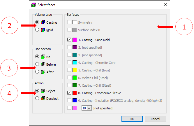
To select the boundaries of one or more indices, check the corresponding lines in the right part of the window (1). Only those boundary indices that are used in the model are available for selection. Borders with indices 10-18 are checked using a special edit box with arrows. Radio buttons (2) indicate where to select the boundaries of the selected indices - in the casting or in the mold. Depending on the selected volume type (2), the list of boundaries indices available for highlighting (1) changes. Radio buttons (3) set how to select boundaries, selected in (1) indices and located in specified (2) volumes, in relation to the section plane. Either all boundaries satisfying conditions (1) and (2), or their part located before or after a given section plane can be selected. To use condition (3), you must first set the section plane to the desired position. How to control the section plane is described in the Section Plane section. Finally, the radio buttons (4) specify the operation itself over the given group of borders – select or cancel selection.
The additional checkbox Only visible (5) applies all filter settings only to those borders that are currently displayed in the workspace. If the setting is enabled, the borders of hidden model elements (whose display is disabled) will not be selected.
It should be note that the face of an element is considered to be located on one or another side of the section plane if all three of its vertices are located there.
After the conditions are set, click the OK button in the Select Boundaries dialog to perform a selection of the boundaries.
Another way to select boundaries is interactive, using the left mouse button and holding down the Ctrl key. In this way, you can select either single element faces or entire surfaces.
|
Switching between selection modes is carried out by the Select Contiguous button on the Edit toolbar. |
If the button is not pressed, the outer edges of the elements are selected one at a time (see the figure below). When the Select Contiguous button is pressed, a mouse click with the Ctrl button pressed will select the entire surface (see the figure below). To deselect individual faces or surfaces use the right mouse button while holding down the Ctrl key.
 |
 |
Selecting individual faces |
Surface selection |
When the Select Contiguous button is pressed, a surface is considered to be a set of adjacent faces, where the dihedral angle between adjacent faces is not less than the specified value in the range from 0 to 180 degrees. For example, if you set this angle to 180°, the adjacent faces that lie in the same plane will be selected, and if the value is 0°, all the faces of the volume will be selected. The default surface angle is 150°.
|
The angle value for the surface, as well as the appearance of the marked boundaries, can be set in the Settings window on the Mark Parameters tab, which is opened by the Mark Parameters button on the Edit toolbar (for more details see Mark Parameters section). |
|
The marked boundaries can be assigned a new index. To do this, click the Assign Boundary Index button on the Edit toolbar. The Boundary Index dialog will open (see the figure below). |
Select the desired item in the list, then press the OK button. The marked boundaries will be assigned the selected index and deselected (see the figure below).
|
All borders can be deselected either by clicking the Deselect All Boundaries button on the Edit toolbar, or by using the Ctrl+G keyboard shortcut. |
 |
To see the result of assigning boundary indices, you can turn on the GM rendering by boundary indices by clicking the Show Boundary Indices button on the Modes toolbar (see details in Model Display Modes section). |
Mathematical models used in POLIGONSOFT impose rather stringent requirements on the quality of meshes, therefore, quality control of elements is an important task of preparing a model for calculation. Ideally, all elements of a tetrahedral finite element mesh should have the shape of a regular tetrahedron, i.e. to the tetrahedral pyramids, consisting of equal equilateral triangles. In practice, this is unattainable, but it should be ensured that the grid does not contain elements with a highly distorted shape - the grid must be fairly regular. In addition, elements whose volume is zero or close to zero - the so-called degenerate elements - are unacceptable. The presence of even one degenerate element can make the calculation impossible. Therefore, the Master module contains functions for improving the overall quality of the mesh and correcting individual "bad" and degenerate elements. In practice, correction of the shape of an element can almost always be done only at the expense of degrading the quality of the elements surrounding it. Therefore, the algorithms for correction cannot be applied to a large number of elements at the same time. And vice versa - regularization algorithms are effective only when there are a large number of vertex elements (i.e. mesh nodes) which can be freely moved.
Mesh quality control and the correctness of the elements is maintained by a group of buttons on the Edit toolbar.

A "bad" element is one that has too small and/or too large dihedral angles. Both mean that the shape of the element is far from correct, it is degenerated almost to a flat figure. Such an element will not be accepted for calculation in the Fourier and Hooke solvers. In addition, solvers impose a number of size requirements on finite elements and the ratio of volume and surface values. These requirements are dictated by the numerical calculation method, they cannot be changed.
|
To edit the limit values for the angles of elements that determine the quality of the mesh, click the Mark Parameters button on the Edit toolbar (for more details, see the Mark Parameters section). |
|
The simplest and at the same time favor way to improve the quality of the mesh as a whole is the performing the Regularization function on the Edit toolbar. |
With regularization, an attempt is made to bring the shape of all finite elements of the model closer to a regular tetrahedron. If the task of the functions of correcting "bad" elements (discussed below) is to avoid their presence even at the expense of some deterioration in the shape of neighboring elements, then the main task of regularization is to improve the quality of as many elements as possible without deteriorating the quality of others. In addition, during regularization, the nodes lying on the boundaries of the volumes, on the position of which its shape depends, remain stationary.
Regularization can be performed multiple times and the mesh quality can be improved. The function works automatically, without user intervention. You can evaluate the results of regularization by the quality histogram, which appears automatically upon completion of the operation (see the figure below).
The mesh quality histogram shows the percentage distribution of finite element dihedral angles over angle intervals. The width of the interval can be changed using the field located above the histogram from 1 to 60 degrees.
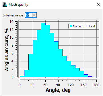
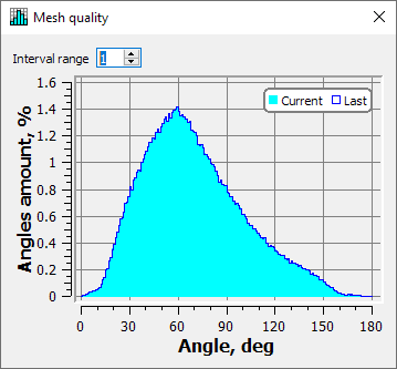
The filled columns show the distribution of dihedral angles after regularization, and the outlines show the distribution of dihedral angles before regularization. The legend is shown in the upper right corner of the diagram. In a good quality mesh, most of the dihedral angles should be close to 70 degrees in magnitude. The diagram is refreshed each time the regularization is performed.
The color of the columns of the chart is the same as the color of the element marks. To change the color of the diagram, use the Special Colors button on the Standard toolbar (for more details see Special Colors section).
|
The angle distribution histogram can be viewed by clicking the Mesh Quality button on the Edit toolbar. |
Another way to improve the quality of the mesh is to reshape only the bad elements. In this case, the algorithm automatically moves the mesh nodes, trying to eliminate invalid geometric parameters in individual, selected mesh elements.
|
To find and select bad elements with angles outside the limit values, you should execute the Check Mesh Quality command on the Edit toolbar. |
When the command is executed, it starts checking the angles and volumes of the casting and mold elements. Then the Check Mesh Quality dialog opens (see the figure below) and the check results are displayed in the table.
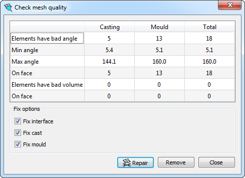
The first column shows information about the mesh quality of the "casting" type bodies , the middle column shows information about the mesh quality of the "mold" type bodies, the third (right) column of the table shows summary information.
For each type of volume, the table shows the following information:
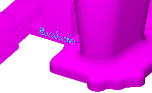
Found bad elements will be selected (marked) in accordance with the previously set label parameters (see the figure below).
The correction of the marked bad elements is started by clicking on the Repair button in the Check Mesh Quality dialog.
The correction process is a responsible operation, since the movement of grid nodes applies to any "bad" elements of the model, including those located on the boundaries. This means that the operation may distort the shape of the object. Therefore, in the lower part of the Check Mesh Quality dialog, there are options for the algorithm for correcting elements (more precisely, shifting mesh nodes). By enabling and disabling the corresponding parameters, you can choose where to allow the displacement of nodes (in the casting, in the mold) and enable or disable the displacement of nodes at the boundaries. The last option allows you to keep the shape of the bodies without distortion.
It should be note that the maximum effect can be obtained when all types of fixes are allowed (enabled by default). The only drawback is the possible distortion of the boundaries of the casting or mold. It is better to run the simulation with some geometry inaccuracies than rebuilding the finite element mesh.
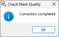
Correction of elements ends with a message (see the figure below). The information in the table of the Check Mesh Quality dialog will be updated.
If, after correcting the elements, the information in the table shows that not all elements with bad angles or degenerate volumes have been corrected, it is advisable to repeat the correction procedure again. It should be repeated as long as the number of detected "bad" elements continues to decrease. If after the next cycle the number of "bad" elements has not decreased, further attempts will be useless.
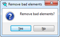
Elements that could not be repaired can be removed from the model. To do this, press the Delete button in the Check Mesh Quality dialog. After confirming the operation (see the figure below), the marked elements are deleted from the geometric model without the possibility of restoration.
Thus, there will be no more bad elements in the model, but the model itself will slightly lose its geometric accuracy.
Attention! Removing bad elements from the model should be done only after the volume types have been specified and the correct bounding indices have been assigned.
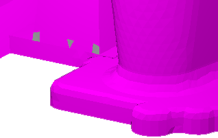
When bad features are removed, the faces of adjacent features become external. However, these faces will have an index of 0 (inner face, see the figure below), which contradicts the accepted "standard" indexing of outer boundaries (usually these are indices 17 and 18). The standard numbering of borders is discussed in the Basic concepts: Volumes, Types, Indices section.
If, after removing bad elements from the model, you change the type of any volume, you will be prompted to assign “standard” boundary indices to all volumes. This can have irreversible consequences. you cannot assign standard boundaries after deleting "bad" elements, so you should click the No button in the message box. If you click Yes, outer boundaries appear in the body of the casting or mold where the feature was removed, resulting in incorrect calculation of temperature fields in that area. It is important to preserve the outer boundaries with the index 0 in such places, this minimizes the calculation error, the system will assume the presence of a virtual element beyond such a boundary.
If, after removing "bad" features, gray faces appear on the outer boundaries of the casting or mold, you can optionally assign them indices of the boundaries with the environment using the tools described in the Editing Boundary Indices section.
|
Additional options for transforming finite elements are provided by the Split Elements command on the Editing toolbar. It becomes available after selecting any group of finite elements and opens the Split Elements dialog (see the figure below). |
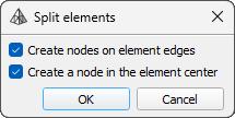
In the window, you can select one of two schemes for the selected mesh elements.
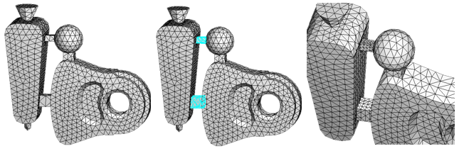
After pressing the OK button, the mesh refinement operation will be performed. An example of mesh refinement in the casting block feeders is shown in Fig. below.
It should be note that the refinement, especially repeated many times, can lead to a deterioration in the quality of the mesh due to the appearance of elements with angles that go beyond the specified maximum and minimum values. In this regard, it is highly recommended to check the quality of the mesh after grinding it and correct the “bad” elements as described above.
In investment casting, the melt is poured into a mold made by alternately wetting the master model with a binder and sprinkling it with bulk material. The result is a casting mold that has an arbitrary shape on the outside and an internal cavity that exactly repeats the geometry of the master model. Building such shells in a CAD system is a laborious process, so the Master module has a special tool for their automatic creation.
The shell is generated for all volumes displayed in the work area, i.e. before creating it, you must turn off the display of bodies in the model tree for which the shell will not be built. In addition, it may be necessary to set a special border index on surfaces where the shell is not needed. For more details, see the descriptions of the respective parameters below.
|
The Create Shell command on the Edit toolbar opens a dialog box where you can set the thickness and other parameters of the shell. The parameters of the finite element mesh of the shell can be selected automatically by the algorithm, or set by the user. By default, automatic selection of parameters is used (see the figure below). |
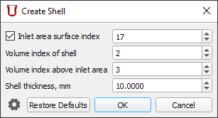
In automatic mode, the following shell parameters are set in the window:
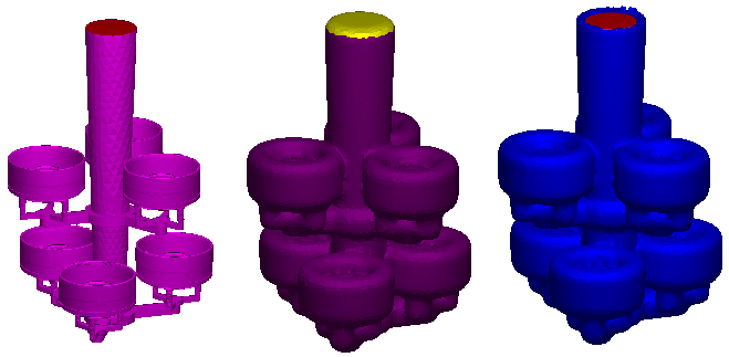
The shell generator is started by pressing the OK button. While it is running, a progress bar is displayed in the status bar. Upon completion of generation, the model will be loaded into the working area of the module.
The whole process of building the shell is recorded in the log files, in case of an error or in the event of a process failure, they can be viewed and sent to the developer. To do this, go to the folder for storing the log files through the Help → Show Logs menu, find the folder with the name containing the date and time the module was started and examine the contents of the files "shell_builder _ *. log" and "shell_builder _ *. err".
After construction the shell, it is necessary to remove the volume above the melt feeding boundary and perform the operation of assigning the standard boundaries (for more details, see the Editing Boundary Indices section).
After building the shell, its quality must be checked with the standard procedure of the Master module and, if necessary, correcting the bad elements. For more information about checking the quality of the mesh, see the Mesh Quality Control section. If the number of bad elements exceeds reasonable limits and cannot be corrected, it is recommended to delete the shell and repeat the operation of creating it, switching to the custom mode for controlling the shell mesh parameters.
|
The Settings button in the lower left corner of the Create Shell dialog opens the preprocessor settings window, where advanced parameters are located that control the shell creation algorithm (see the figure below). |
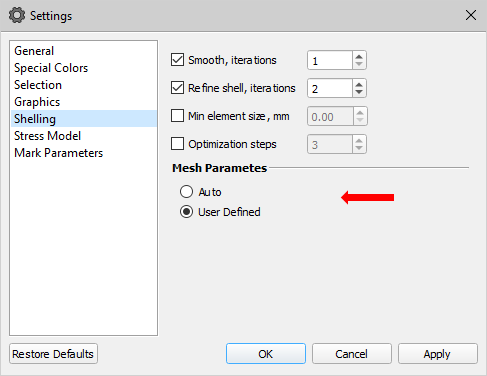
These parameters control the operation of the mesh generator and affect the quality of the resulting shell. Most of them are optimally tuned and do not need to be changed unnecessarily. The exception is the Mesh Parameters group, where the Auto and User Defined switches are located (marked in the figure above). By default, the automatic selection of parameters is set. If you go to the User Defined mode and then click the OK button, the appearance of the Create Shell dialog box will change (see the figure below).
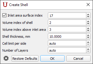
In this mode, when creating a shell, the user can specify two more parameters. By default, both parameters are in the "auto" mode, which means that they are set by the algorithm automatically (which corresponds to the automatic mode). By setting the parameters to specific values, you can control the mesh quality and achieve the desired results.
The procedure of shell creation can be repeated as many times as necessary to obtain multilayer shells with different properties. For example, in this way, first a model of a ceramic mold can be created, and then a model of thermal insulation wrapped around the mold. For more complex insulation, some layers of thermal insulation can be cut off by editing the volume indices (see details in Editing Element Indices in the Arbitrary Areas section).
In the Master module, you can create new volumes or modify the geometry of existing volumes by extruding a surface or part of it. This can be an extremely useful option when there is a need for a minor and relatively simple GM change. In this case, there is no need to change the original CAD model, then re-generate the FE mesh and import it into POLIGONSOFT. You can easily change the dimensions of the risers of a simple form, create layers of thermal insulation, covers, change the geometry of the casting, etc.
The created new volume is a mesh of the specified thickness, obtained by offsetting the selected surface. Therefore, before starting extrusion, you should mark the required surface or part of the surface (for methods of marking boundaries, see the Editing Boundary Indices section). As an example, let's increase the outer diameter of the pipe by 2 mm. In fig. below the outer cylindrical surface of the pipe is highlighted (the body has the "casting" type).
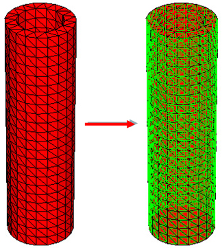
|
The Extrude Mesh button on the Edit toolbar calls a dialog box in which the thickness of the future shell is set in mm (see the figure below). |
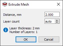
The window specifies the distance in mm by which the surface mesh should be extruded and the number of mesh layers that will be created in this case. By default, the second parameter is set to "auto", which means that the required number of layers will be calculated based on the size of the elements of the original mesh and the distance by which it will be extruded. The "auto" value can be changed to the desired one, then the layer thickness will be recalculated and the value will be shown in the information field.
After clicking the OK button, the operation will be performed, a new volume of the "mold" type will be created with a certain volume index that is different from the parent body (see the figure below).
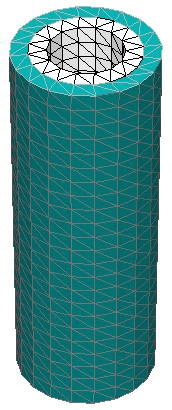
Now you can change the type, volume index and other parameters of the new volume, achieving the desired result. For example, following the purpose of the example, you can set the new body to a "casting" type and merge it with the pipe body, which will change the geometry of the casting.
|
Model Information button opens a window that contains information about the loaded geometric model. To call the command, you can use the key combination Ctrl + I (see the figure below). |
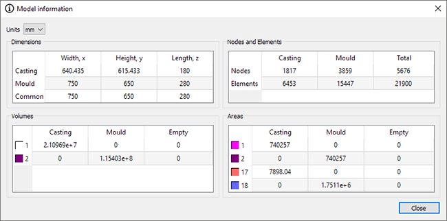
The window displays the following information:
The units in which the information is displayed are specified in the list in the upper left corner of the window (by default - meters). If necessary, the values of the table cells can be copied to the clipboard. To do this, you need to make two clicks on the cell to make it active, after which the copy function will become available.
You can close the information window by clicking the Close button in the lower right corner of the window.
POLIGONSOFT can simulate the filling of a casting mold with melt and other flow-related problems. The calculation is performed by the Euler solver, which solves the problems of melt flow and its temperature change during interaction with the mold and the environment, including solidification. The following results can be obtained as a result of the calculation:
Additionally, Euler solver can be used to evaluate the gating system operation without considering the casting body.
The problem of predicting shrinkage cavities, macro- and microporosity is not solved at this stage.
To perform the calculation of mold filling, the following data are used, prepared in the Master module:
The Preparing the Modeling Area section describes the general principles of preparing the model for calculating the temperature field and shrinkage porosity. The case of mold filling simulation requires additional preparation of the geometric model in the Master module.
Usually, the mold is filled with melt from a ladle. To simulate this process on the casting surface, it is necessary to specify the area (or areas) through which the melt will flow. This can be done using the special tool Inlets.
|
The Inlets button on the Edit toolbar opens the editor (see the figure below), in which the parameters and the order of filling the casting are set. This data can be applied to solve one specific problem or exported to a bdv file for use in other calculations, including as a process template. |
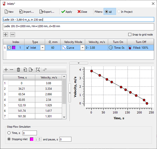
The window contains a table of regions (inlets) through which the melt is fed into the mold cavity (more precisely, into the casting body). Under the table there is an area for editing curves and parameters that control the stop of the solver.
To create a inlet, press the "+" button above the table on the left. The first row appears in the table. By pressing the "+" button you can create no more than 9 inlets. To delete an unnecessary inlet, select it in the table and press the "-" button above the table on the left, the line will be deleted from the table.
After the inlet is created, it needs to be configured. Since the inlet is a virtual stream of the melt, you need to set its dimensions and the entry point on the casting surface. It is assumed that the jet is in the shape of a cylinder, so its size is given by the diameter of the circle. Left-clicking with the Ctrl key pressed on the casting body starts drawing a circle, which denotes the melt stream (see the figure below). The center of the circle is set by the mouse pointer.
To the right of the table is the Snap to mesh node option. When this parameter is enabled, the center of the stream is always at the mesh node. When the parameter is deactivated, the center of the stream is displayed at random. It is recommended to enable this parameter if the melt inlet is specified at the symmetry boundary, this will avoid errors when calculating the area of the stream.
In the inlet line, you can set the parameters that determine the operation of the inlet (see the figure below).
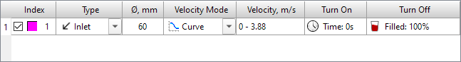
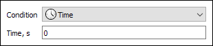
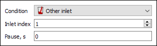

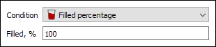
After the Inlets are set, press the OK button. The dialog box will be closed, but the Inlets outlines will continue to be displayed on the model.
As an example of the use of several inlets, consider the technology of filling a form through a riser with topping up in two risers (see the figure below).
The main inlet # 1 supplies the melt to the downsprue from the beginning of the calculation (from the zero second of the process). When the form is half full (the condition for turning off the feed - 50% of the filled volume), inlet # 1 is turned off, followed by a pause of 2 seconds, during which the ladle moves towards the inlet # 2, set on the surface of the first riser. In 2 seconds after the end of the first inlet , inlet # 2 starts to work - the melt is added to the first riser. It ends when the form is 3/4 (75%) full, then a pause of 2 seconds follows and inlet # 3, set on the surface of the second riser, begins to work. Inlet # 3 finishes work when the form is completely filled out.
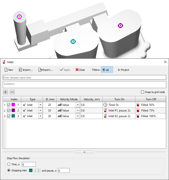
For each inlet, the velocity of the incoming melt is set. The velocity can be set by a constant value or by a speed-time curve.
In most cases, the flow calculation is stopped (followed by switching to the solidification and porosity calculation) when the mold is completely filled or when all Inlets are turned off. This situation is automatically tracked by the preprocessor and the solver and no additional parameters need to be specified. In cases where the moment of stopping the flow calculation cannot be determined automatically, it is required to specify it manually in the Stop Flow Simulation group. See the section below for more information.
In some problems, at the beginning of the calculation, there are volumes filled with melt. For example, it can be a pre-filled sprue bowl from which the melt is poured into a mold or crucible of a melting plant during vacuum casting. In such a situation, it can be inconvenient to set the flow of the melt into the mold using the inlet. To simulate the melt flow, an appropriate geometric model must be prepared, in which the pre-filled volume or volumes will be present.
If the container, for example, the ladle at the beginning of the calculation is not completely filled, its model should be prepared, consisting of two parts - filled and empty, or only the filled part of the bucket should be used in the calculation (see the figure below). In any case, the pre-filled volume must be of the "casting" type and have a separate index (in the figure below it is the volume with index 9, red).
The selected volume index should be marked as “filled” in the model tree. To do this, left-click on the empty glass icon to the right of the bucket volume (in this example, this is index 9). In this case, the icon will change to the image of a full glass. To undo the changes, you need to click on the icon again. If the model contains multiple casting volumes with the selected index, all of these volumes will be marked as filled, so it is important to set a unique index to the filled volume. In general, you can specify several filled volumes, and they can have different indices, but you cannot specify as filled one volume from a group of volumes with the same index.
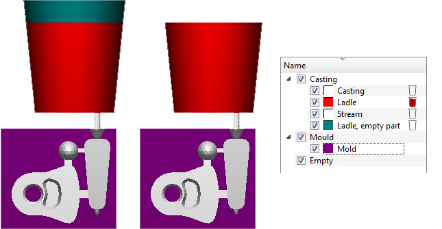
If a prefilled volume is specified in the model, this is a sufficient condition to run the Euler flow solver; you do not need to specify melt inlets. However, if the problem statement requires it, leads can be specified as usual in the required quantity as described in the previous section.
In most cases, the flow calculation is stopped (followed by switching to the solidification and porosity calculation) when the mold is completely filled or when all the inlets are turned off. This situation is automatically tracked by the preprocessor and the solver and no additional parameters need to be specified. In cases when the moment of stopping the flow calculation cannot be determined automatically, it is required to specify it manually in the Stop Flow Simulation group. See the section below for more on this.
At a certain moment in time, the Euler flow solver stops working and further calculations are performed by other solvers (if specified in the simulation parameters). In most cases, this happens when all inlets finish their work, for example, when the mold cavity is completely filled with melt. There are situations when the desired moment of switching between solvers does not coincide with filling the mold, here are some of them:
In order to flexibly control the moment of stopping the flow solver and switching to the calculation of solidification and porosity (if specified) in the Inlets dialog there is a Stop Flow Simulation group, where you can select one of two criteria that stops the work of the Euler solver (see the figure below).
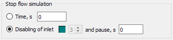
Consider the criteria for stopping the Euler flow solver.
Calculation of casting solidification taking into account heat exchange with mold elements and the environment, as well as pipe shrinkage and macro- and microporosity prediction - the main task of the casting process simulation, performed in the Fourier solver. As a result of the calculation, the following results can be obtained:
Note. At the beginning of the solidification calculation, the mold is filled with melt. The filling problem is solved by the Euler module (see the corresponding section).
To perform the majority of temperature fields, solidification and shrinkage porosity calculations, in addition to the prepared geometric model, the following data are required, which are need to be prepared in the Master module:
A detailed description of all parameters is given in chapter 6 in Thermal and Porosity Simulation section.
To simulate special casting processes (vacuum casting, continuous casting, high and low pressure die casting, etc.) additional data may required (see relevant sections).
POLIGONSOFT allows modeling the stress-strain state (SSS) of a casting and a mold, taking into account their contact interaction. The calculation of stresses and strains is performed by the Hooke solver based on the results of a previously made thermal calculation using the Fourier solver. The following results can be obtained as a result of the calculation:
As a result of the work of the Fourier thermal solver, files are written that contain the temperature fields of the casting and the mold. These files are part of the initial data for the work of the Hooke solver.
To calculate SSS, you need the following data, which are prepared in Master and Mirage (optional) modules:
Preparing the Modeling Area section describes the general principles of preparing a model for calculating the temperature and porosity field. The task of modeling the SSS requires additional preparation of the geometric model in the Master module.
First of all, thermomechanical properties of materials must be specified for all volumes involved in the stress calculation. They are specified in the Material Properties editor on the Stress tab. The set of thermomechanical characteristics describes the behavior of the material when its temperature field changes and is called the Thermomechanical Model. Two thermomechanical models are available for the casting material, they are selected from the list in the first row of the table (see the figure below):
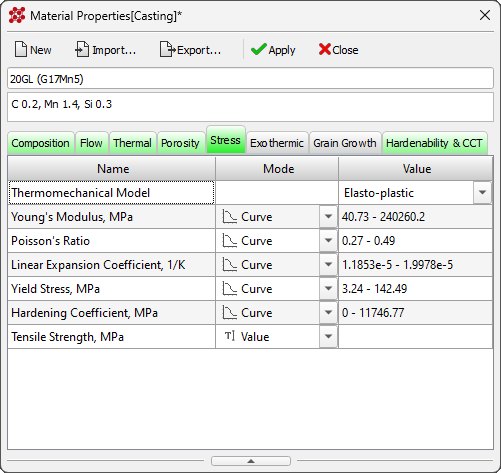
For most cases, the Elasto-plastic model is suitable; it requires specifying the entire set of parameters. In some cases, it is permissible to use a Linear Elastic model of material behavior for casting (see the figure below). This is a simpler model, it is suitable for cases when the body is always in a solid state and its temperature changes insignificantly and the heating-cooling cycle does not lead to an irreversible change in shape and size.
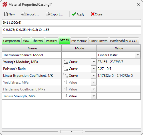
In the current version of POLIGONSOFT, only one thermomechanical model can be used for a mold, regardless of the number of materials used in it. The behavior of the mold is set by the calculation parameter Contact Interface with Mold in the Start Simulation and Parameters window on the Stress tab (for more details, see the Stress Simulation Parameters section). There are several options available for the interaction of the casting with the mold:
The first two models do not require any thermomechanical properties. This means that even if such properties are specified, they will be ignored. The other two models require that thermomechanical properties be specified for the mold. When selecting the type of contact interaction with the mold in the Start Simulation and Parameters window, you will also need to set the Mold Stress Properties Volume Index parameter there. The parameter specifies the volume index of the mold to which the material properties are tied and its thermomechanical properties will be used when calculating stresses. Thus, when selecting the interaction of a casting with a linear-elastic or elastic-plastic mold, thermomechanical properties are used only from one material specified in the Mold Stress Properties Volume Index parameter. In this case, it is not necessary to switch the thermomechanical model in the material properties; it is enough that all the necessary properties are specified.
Some mold materials can be excluded from the calculation. For example, if the interaction of a casting with an absolutely rigid or linear-elastic metal or sand mold is calculated, then the mechanical impact of such materials as fibrous refractories, wools, burnt-out exothermic sleeves can be ignored. Such mold materials can (and should!) be excluded from the SSS calculation, while their role in the formation of the thermal picture is preserved. To do this, check the box Empty for Stress for the selected volume indices in the Volume Parameters window, or click the mouse in the model tree in the corresponding cell opposite the desired index (see the figure below). Volumes not involved in the SSS calculation are considered "empty" from the point of view of the thermomechanical problem and are marked with an icon in the model tree.
Note: Only volumes of the Mold type can be marked empty.
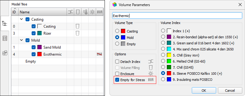
The stress-strain state of the casting at the end of solidification is generally determined by the history of the temperature field of the casting and its contact with the mold. This state is not final and may differ significantly from the stress-strain state of the casting removed from the mold and freed from the elements of the gating-feed system (GFS). Thus, in order to understand what the final geometry of the casting will be and how the residual stresses will be distributed in it, it is necessary to calculate the stress-strain state after removing the casting block from the mold and then after removing the GFS elements.
To calculate the change in SSS when removing collectors, risers, etc., these elements of the model must have unique volume indices. It is best to split the model into separate bodies at the stage of its preparation in the CAD system, but in extreme cases, you can split the casting mesh into parts using the Master tools described in the Editing Element Indices in the Arbitrary Areas. section. As a result, the casting will consist of bodies with different indices, while index 1 is always assigned to the casting itself, i.e. the part that remains and cannot be deleted (see the figure below).
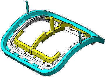
The moment of removing the casting from the mold and the order of removing the elements of the gating system are specified in the calculation parameters (for more details, see the sections Stress Simulation Parameters and Stress Simulation at subsequent technological stages).
Radiation heat transfer can be considered on the basis of a simple expression for the heat flux (Stefan-Boltzmann law) or calculated using a complex algorithm that takes into account the effects of radiation energy reflection and shading of some bodies in the computational domain by others. Such a model for calculating radiation heat transfer used in POLIGONSOFT does not take into account the influence of the environment, i.e. the heat transfer coefficient to the environment and its temperature (including the dynamic medium) are not taken into account.
A problem involving complex radiation heat transfer requires special preparation of the geometric model and, in some cases, special process conditions, for example, the translation mode that sets the movement of bodies when modeling directional crystallization (for more details, see the Translation Modes section).
Since radiation heat transfer involves the calculation of the interaction of parts of the geometric model (casting and mold) with the surrounding bodies (for example, a melting unit, a mold heating furnace,...), it is necessary to include these bodies into a geometric model. You should remember that it is recommended to create a closed computational domain. For example, if the casting is placed in a vacuum melting plant, the computational domain will include: a casting, a mold and a vacuum melting plant body surrounding them.
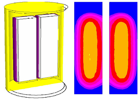
a) b)
In the above example, the entire geometric model is included in the computational domain. However, it can only include part of the geometric model. Consider a more general (and more complex) case: a mold with a melt is placed in a mold heating furnace. Part of the form goes beyond its limits. It can be assumed that for the part of the mold that is in the furnace, the influence of the environment (air) is insignificant. Most of the heat is transferred by radiation. On the other hand, this cannot be said for the part of the form that goes beyond its boundaries. The task can become more difficult if the furnace has a movable bottom. Then, when the casting moves in the vertical direction, the area located in the zone of radiation heat transfer changes in time. Consider two options for configuring the computational domain.
Option 1. The geometric model (file g3d), in addition to the casting and the mold, includes a model of the mold heating furnace and the enclosing body – Enclosure, which simulates the walls of the vacuum melting plant or other surrounding space that closes the computational domain (see figure below). In this case, the boundary of the radiation heat transfer computational domain by is set according to the Enclosure. If the mold heating furnace and the casting move relative to each other, a curve (or curves) of their movement is specified (for more details, see the Movement Modes section).
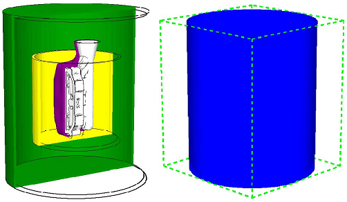
a) b)
Note. The shape and size of the Enclosure can significantly affect the accuracy of the simulation results. For example, when modeling radiation heat transfer in a vacuum melting plant, it is important to accurately convey the shape and dimensions of its internal space.
Option 2. In the geometric model (.g3d file), in addition to the casting and the mold, only the model of the mold heating furnace is included. In this case, the boundary of the radiation heat transfer region is set by the heating furnace (see the figure below). If the mold heating furnace and the casting move relative to each other, a curve (or curves) of their movement is specified (for more details, see the Movement Modes section). The difference from the first option is that for those parts of the mold and casting that go beyond the boundary of the computational domain (over the heating furnace border), the calculation will be carried out according to the usual heat exchange rules with the environment. The coefficient of heat transfer to the environment, emissivity and the environment temperature, specified in the heat transfer parameters, will be taken into account (for more details, see Heat Transfer Parameters section). It should be note that with this version of the problem setup, the part of the casting block located outside the ray tracing boundaries (outside the mold heating furnace) does not participate in radiative heat transfer with energy reflection effects, which can be a rather serious deviation from the real situation. For example, in the described example, the part of the mold that is outside the heating furnace will not “feel” its (furnace) influence.
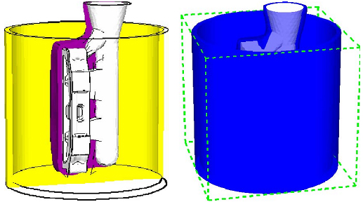
а) б)
The first option corresponds to a more accurate formulation of the problem, since in reality the radiation of the heating furnace also affects the parts of the block protruding from it. The second option can be used when it is necessary to take into account the exit of the mold from the radiative heat exchange zone with a change in the heat transfer model, for example, when the mold moves in a vacuum melting unit and is immersed in a liquid metal cooler or other medium. In this case, the accuracy of the calculation may suffer due to the creation of a clear virtual boundary that the radiation cannot "surpass". (see the figure below).
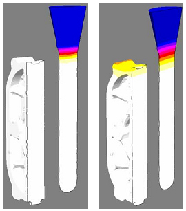
a) b)
Let us give an example of an incorrectly specified computational domain. In fig. below, the dimensions of the computational domain are given according to the casting mold. As a result, an open computational domain was obtained - the upper end of the bowl does not have radiation heat exchange with any other surfaces. Due to the specified dimensions of the radiation area, the possibility of heat transfer from the top of the bowl to the environment is excluded. If you carry out a calculation with such a calculated area, then the results obtained will be absolutely incorrect (cooling will go from bottom to top, the metal in the bowl will solidified last).
To set the computational domain for radiative heat transfer, you need to specify a body that plays the role of Enclosure. To do this check the Enclosure checkbox (1) in the Volume Parameters dialog of the selected body (see the figure below). In this case, an interactive icon (2) will appear in the Model Tree opposite the marked body. You can control the enable/disable Enclosure by right-clicking on the icon in the Model Tree.
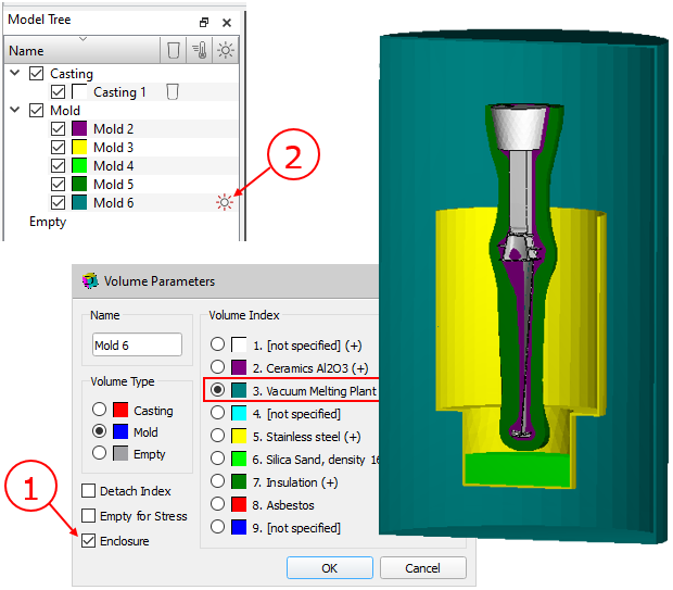
It should be note that Enclosure, like other volume parameters, is assigned to the volume index, so all other bodies with the same index will also be marked as Enclosure.
The volume indices for radiation heat transfer are assigned in accordance with the idea of the calculation. For example, if you want to calculate the cooling of a casting block installed in a metal box and the temperature distribution in it is of interest, you should assign a volume index according to the required material properties (see the Materials Assignment section). If the calculation of the temperature in the Enclosure is not of interest, you can assign a constant or variable temperature to it (for more details see the Temperature Modes section).
Calculation of radiation heat transfer (ray tracing) is performed only between the boundaries with the "default" environment, i.e. between boundaries 17 and 18 in any combination. For each of these boundaries it is necessary to set the emissivity E in the heat transfer file and the parameter Surface Fraction > 0 (for more details see the Heat Transfer Parameters section). If the computational domain includes many bodies with different emissivity: casting mold, sand, thermal insulation, steel flask, etc.), in this case you can set the values of the effective total emissivity, depending on the emissivity of each surface that falls within the raytraced region for boundaries 17 and 18 in the heat transfer file. All types of boundary heat transfer can be taken into account in the heat transfer settings. This will make it possible to solve "mixed" problems that have areas where heat transfer by radiation is calculated taking into account the effects of shading (there is no environment), and areas in which the calculation is carried out taking into account the environment.
If other external boundaries except 17 and 18 are assigned in the radiative heat transfer computation domain, they do not participate in the complex radiative heat transfer, i.e. for them, heat exchange with the medium can be set, including taking into account radiation according to the Stefan-Boltzmann law. This can be used, for example, if it is important to take into account the heating of the walls of the vacuum melting plant from the inside and their heat exchange with the environment from the outside. On the fig. below on the outer walls of the melting plant (given by the Enclosure for the area of radiative heat exchange), boundary 3 is set for which convective heat exchange with the medium is set.
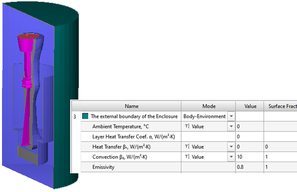
To reduce the calculation time, it is reasonable to assign the outer boundaries of the Enclosure body index 0 if the calculation of temperatures in the Enclosure is not performed (see the figure below). You can also assign boundaries with index 0 to some surfaces of the computational domain that do not play a significant role in heat transfer.
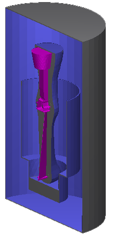
Before starting the calculation, you should enable Radiation parameter on the Solidification tab in the Start Simulation and Parameters window (for more details, see the Thermal Simulation Parameters section). This parameter launches a special module that is used to calculate ray tracing between objects, incl. moving. The module uses as source information a .g3d geometry file, in which at least one volume index is set as Enclosure, a .mve movement modes file (if specified) and creates a .rad file based on them, which contains not only the FE mesh, but also information about which surfaces (triangular facets) "see" each other and which "do not see" in each specified moment in time (the so-called view factors). If the volumes of the model do not move, the view factors do not change during the calculation. However, if the bodies are assigned movement modes, the view factors must be calculated for different positions of the bodies relative to each other. Further, the .rad file is used by the Fourier solver.
The solution to the problem of saving metal while maintaining or increasing the efficiency of casting feeding can be achieved by using mold materials that insulate or give off heat to the riser zone. When modeling the conditions for manufacturing a casting in a mold containing special heat-insulating materials, to take into account their effect, it is enough to set the necessary thermophysical properties in the corresponding volume of the 3D mesh model. The case of modeling the casting formation in the presence of materials from an exothermic (thermite) mixture requires the use of a special model, which includes a description of the conditions for starting a reaction during thermal interaction of a material with a liquid metal, its dynamics with active heat release.
The decision on the need to use exothermic materials is made when developing or optimizing a foundry technology, based on considerations of economy and the possibility of ensuring the required quality of castings. In a number of cases, the installation, in particular, of exothermic sleeves of the risers may be the only available option to ensure continuity in the feeding zone of the casting due to the structurally determined insufficient size of the platform for placing the risers. When initially choosing the size of the riser sleeve (see figure below), the concept of its module (equivalent to ordinary riser) is used to select a specific model from the proposed size range. Subsequent adjustment of the decision made can be carried out based on the results of the analysis of its effectiveness in POLIGONSOFT.
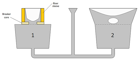
Riser sleeves can be supplied complete with sandy breaker cores attached to the bottom of the sleeve to form a thinned section of metal - the riser neck. This reduces the labor intensity of separating the riser from the casting and reduces the amount of machining in the corresponding area. With the correct choice of the width of the riser neck, formed by the central channel of the breaker core, the liquid metal feeding does not stop during the entire time of operation of the riser. In this case, premature solidification of the riser neck does not occur due to its strong heating and low heat removal from the breaker core.
In most cases, exothermic sleeves are made from a bonded mixture of powders or shavings of aluminum and iron oxide with additives. In contact with the melt, such a material ignites when relatively low temperatures of several hundred degrees are reached. The oxidation reaction is accompanied by intense heat release (Q): Fe2O3+2Al®Al2O3+2Fe+Q. For a relatively short time of the reaction in the sleeve volume, the released heat makes it possible to heat the riser, create a strongly heated zone around it, including the area filled with reaction products, and the adjacent mold. In most cases, the sleeve retains its coherence after completion of the reaction, which allows it to work already as a loose, effectively insulating material, and also facilitates measures to prevent clogging of the recycled mixture.
To simulate the exothermic sleeves behavior during casting solidification, POLIGONSOFT implemented a common adapted model, when the sleeve material has a set of effective thermophysical properties, including the heat of transformation. When using this approach, it is possible to simulate with sufficient accuracy the conditions of thermal behavior of the material without calculating the reaction of interaction between the components of the exothermic mixture. In this case, the effective thermal properties of the material are tied to the model and size of a particular sleeve or their family and include a “correction” associated with phenomena that cannot be taken into account when solving the Fourier equation (1).
|
(1) |
where t – temperature; |
|
(2) |
where m – converted substance fraction, which varies from 0 to 1 for a fixed time for the |
Initially I=0. The moment of activation of the heat source in the sleeve mesh node is determined by the ignition temperature tign, which starts the counter of the increment of the current reaction time τr (from 0 to τign) and the fraction of the converted substance. Heat release stops at m=1, the mixture in this area is considered "burnt out" (3).
|
(3) |
The initial data for solving equations (1) and (2) are the given properties of the material C(t), r(t), l(t), L, and m=m(tr); m set on the interval [0, 1] as a function dependent on the reaction time tr on the interval [0,tign].
Type III boundary conditions apply at the contact between the sleeve and the metal, the mold, and the environment. The heat transfer coefficients along the boundaries with the metal and the mold can also be included in a set of individually specified special data due to the special characteristics of the sleeve surface.
To calculate the foundry technology using exothermic materials, the model prepared in the Master module must contain their volumes (see the figure below), which are assigned indices in accordance with the specified materials or the loaded process template (mold materials properties file). For more information about indices and materials, see the Basic concepts: Volumes, Types, Indices и Materials Assignment sections .
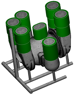
In the example shown in Fig. above, the volumes of sleeves are assigned volume index 7, for which the properties of the exothermic material should be specified. For such a material, in addition to the usual set of properties specified on the Thermal tab in the Material Properties editor, you should enter parameters that specify the conditions for the thermite reaction to occur (see the figure below). They are set on the Exothermic tab (for more details, see the Material Properties section and the corresponding subsection).
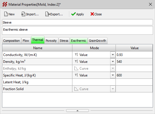
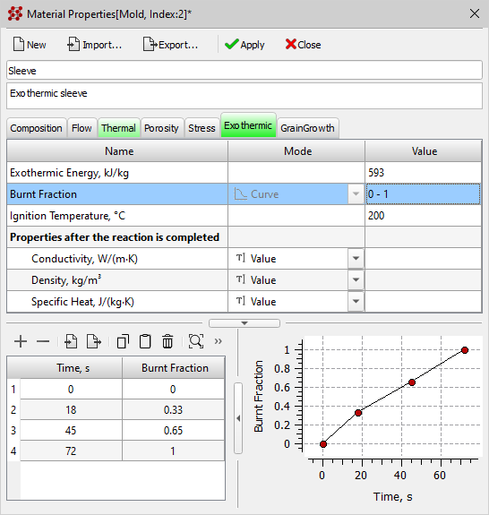
The exothermic materials properties can be set by the user based on their own data or loaded from the database, from the %POLIGONSOFT%\Database\Exothermic folder.
By default, the heat transfer between the casting and the exothermic sleeve is set in the same way as between the casting and the sand mold, i.e. the boundary with index 1 is assigned. There are no boundaries between the sleeve and the mold by default, an equivalent mesh is used, which corresponds to the conditions of ideal contact. To set heat transfer conditions at the casting-sleeve boundary other than those accepted by default, select the corresponding interfaces and set a unique index for them, for which the required conditions must be entered in the heat transfer parameters (for more details, see the Editing Boundary Indices and Heat Transfer Parameters sections). The figure below an example of assigning special indexes on the casting-sleeve and sleeve-mold surfaces is shown.
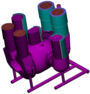
For the boundaries selected in this way, the appropriate heat transfer conditions should be assigned (see the example in the figure below) in the Heat Transfer editor. Parameters can be set independently or imported from templates stored in the %POLIGONSOFT%\Database\Exothermic folder.
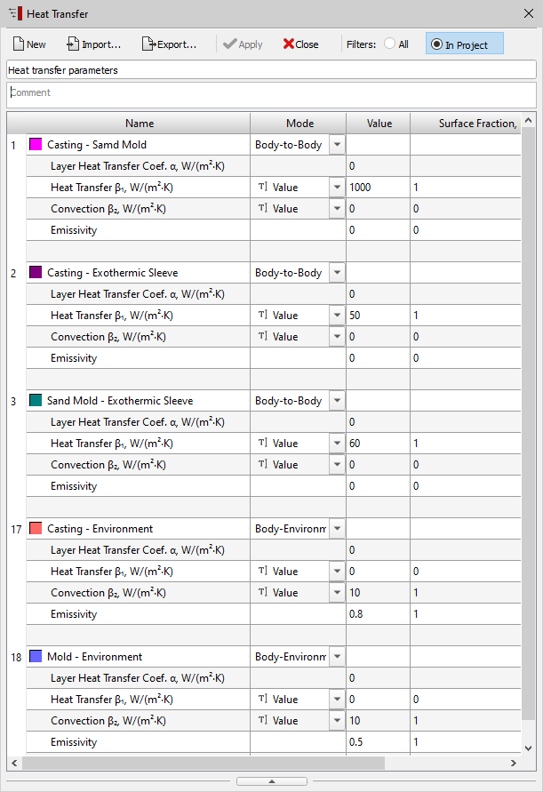
It should be note that in order to set the sleeve-mold interface, it is necessary to separate the sleeve volume index from the mold and set the contact condition between the parts of the mold (for more details, see the Editing Volume Types and Indices). In most cases, you can skip this and work with ideal contact between mold elements.
After entering other parameters of the casting process, set in a standard way, and performing calculations, it becomes possible to observe the thermal history of exothermic sleeves and analyze the effectiveness of their use to provide improved casting feeding (see figure below).
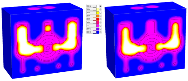
POLIGONSOFT allows you to simulate thermal processes in a mold without its finite element (FE) model using a virtual semi-infinite mold (or virtual mold ). This can be useful, for example, when simulating large sand casting or investment casting using a casting box with sand. The virtual mold can also be used for all types of casting, if the main purpose of modeling is to fill the mold with melt.
When using a virtual mold, it is necessary to specify the properties of its material and the heat transfer coefficient at the casting-virtual mold or mold-virtual mold interface.
Since the volume (FE mesh) of the mold is absent in the model, its thermophysical properties cannot be specified as usual - using the volume index. Instead, the boundary index specified on the outer surfaces of the casting or mold is used, behind which the virtual volume is supposed to be located. In accordance with the rules for using boundary indices (see Basic concepts: Volumes, Types, indices section for more details) indices from 1 to 9 can be assigned to the boundaries between a casting and a mold or a mold and a mold . If such an index is assigned to the outer boundary of the volume, i.e. a surface beyond which there is no other volume, the POLIGONSOFT solvers will assume that a virtual volume of the Mold type is located beyond this boundary. The material properties of the virtual mold will be used according to the boundary index. This rule is true for both casting boundaries and mold boundaries - in any case, the virtual volume will a Mold type. Below are two examples of using a virtual mold.
Example 1. Sand casting. The figure below shows an example of a sand casting in which the volume of the mold is replaced with a virtual one. The full case is shown next to it for comparison. The complete model (right side of the figure) consists of a casting, a mold and a chill plate, a model with a virtual model (the left side of the figure) consists of a casting and a chill plate. In the full case, the volume of the mold with index 3 is given, for which the properties of the sand are set, and the heat transfer parameters are set by the standard boundary with the index 1. In the problem with the virtual mold, sand properties and the heat transfer parameters are set by the boundary with the index 3. In this case, you need to make sure that the heat transfer for boundary 3 is set correctly.
|
|
a) |
b) |
|
|
a) |
b) |
Example 2. Investment casting. In the manufacture of steel castings by the Investment Casting method, the shell mold is usually placed in a box with a sand. Geometry design of a shell mold in a CAD system is a rather laborious task, therefore the preprocessor has a special tool that allows you to create a realistic mesh model of a shell mold (see details in Shells Creation section). However, in this case, the problem of joining the mesh of the sand, which can be designed in the CAD with the shell mesh, which is built without reference to geometric objects. The figure below shows hot to solve this problem using a virtual mold.
In variant a, it is assumed to use completely virtual sand through the designation of a border with an index of 6 on the outer surface of the form (border 6 is selected in accordance with the attached Mold Properties File). The heat transfer coefficient for this boundary (shall-sand) is specified in the heat transfer file.
In variant b, some layer of sand was created using the Create Shell tool. In this case, the thickness of the shell with the sand properties (volume index 6 in accordance with the attached Mold Properties File) is chosen arbitrarily, for example, it can be equal to the distance from the ceramic mold to the bottom of the box, or you can focus on the heating thickness of the sand. In any case, the second shell simulates the heating of real sand, and on its outer boundary heat transfer with virtual sand is specified, as in variant a.
|
|
a) |
b) |
|
|
a) |
b) |
The principle of centrifugal casting is that the mold is filled with melt and the casting is formed by rotating the mold around a horizontal, vertical or inclined axis. This achieves additional impact on the melt and the solidifying casting by the field of centrifugal forces. The process is implemented on special centrifugal machines.
The main feature of the castings formation during centrifugal casting is that the filling of the mold with melt and the solidification of the casting occur under the action of centrifugal forces, which, as a rule, are many times greater than the force of gravity.
There are many different types of centrifugal casting units. In general, centrifugal casting allows for denser castings. In gravity casting, the acceleration vectors of gravity are always directed parallel to each other in one direction. In centrifugal casting, the acceleration vectors are directed from the rotation axis in all directions. This allows for the organization of such formation of thermal hot spots that will more effectively remove shrinkage defects from the body of the part. In addition, since centrifugal forces are significantly greater than gravitational forces, centrifugal casting improves the filling of the mold, provides increased piezometric pressure in the body of the solidifying casting, and a finer structure on the outer surface due to a better contact and more intensive cooling along the outer surface.
The centrifugal casting model used in POLIGONSOFT has the following limitations:
To start the calculation of centrifugal casting, the same data set is required as for gravity casting (sand casting or investment casting).
In this case, the orientation of the model must be set in such a way that the axis of rotation coincides with the direction of the Y axis of the coordinate system. To change the orientation of the model, see the Change Model Orientation, Position and Size) section.
The melt inlet should be set so that its center is located on the axis of rotation (or close to it). For more details on the inlets, see the Melt Inlet section.
|
It is also necessary to set the mold rotation axis and process parameters. To do this, in the Master module there is a special tool Rotation, which is launched with the button from the Process toolbar. |
When the Rotation tool dialog box is open, left-clicking with the Ctrl key pressed on the model starts drawing a circle, the center of which marks the point of the axis of rotation (see the figure below). The direction of the axis of rotation corresponds to the normal to the surface on which the point is located. An arrow on the circle indicates the direction of rotation.
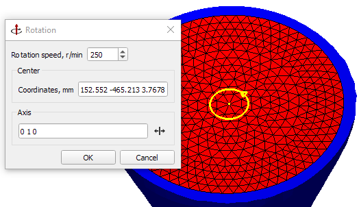
Rotation parameters are set in the dialog box:
 button to the right of the output field of the direction of the rotation axis vector.
After all the rotation parameters are set, press the OK button. The dialog box closes, but the revolve path continues to display on the model.
From the first moments of pouring the molten metal into a sand mold, an uneven pressure field develops within it. In the simplest case (casting into a non-gassing mold), this occurs due to the varying temperatures of the air within the pores of the mixture, located at different distances from the interface with the metal. The situation becomes more complex when the mixture has an unstable structure due to the presence of thermally unstable binders, burnable additives, and moisture, the gaseous products of combustion and evaporation of which are transported into adjacent layers by the pressure gradient.
When unfavorable conditions for gas evolution arise (the presence of cores surrounded by metal without gas venting channels, suboptimal density distribution in the mold with increased density in layers adjacent to gas emission zones, insufficient gas permeability of the mixture as a whole, etc.), a pressure gradient develops, directed toward the casting rather than into the mixture. If at this point there is no solid crust on the casting surface and the resulting pressure is capable of overcoming surface tension forces, gases are embedded in the metal. If they cannot be removed in the liquid phase of the casting, this leads to the risk of gas defects due to mold failure.
Modeling the mold's gas flow allows to identify the potential for gas defects in castings. Calculations allows to monitor the conditions for gas formation and release, allowing us to make decisions about process adjustments, core or mold ventilation, and density control during manufacturing.
In its current implementation, the model allows for the study of gas transfer conditions in a non-gas-forming mold and in a mold with a gas-forming binder (chemical source). Gas transfer processes in the mold are determined in parallel with thermal calculations based on the numerical solution of a differential equation describing the pressure field.
The following fields are available based on the calculation results:
When viewing the calculation results, the following assumptions made in the first version of the gas exchange model implementation in the mold should be taken into account.
To calculate the gas regime of the mold, the following data is used, prepared in the Master module:
The calculation of gas transport in the mold is based on the numerical solution of equation, obtained on the basis of the equations of continuity, Darcy and the ideal gas state:
|
(1) |
| where P – pressure in the pores of the mixture; T – temperature; t – time; Kp – permeability coefficient; m – dynamic coefficient of gas viscosity; m – porosity of the mold material; M – molar mass of gas; R – universal gas constant; I – specific mass of gas released per unit volume of the mixture. |
The derivative  expresses the mass power of the gas release source and, if present, takes on a nonzero value. The description of the conditions for thermal degradation of the binder accompanied by gas release is based on the model:
|
(2) |
| where g – degree of conversion of the binder; f – specific gas-producing capacity; Mb – the initial mass of the binder per unit volume of the mixture (calculated based on its known addition to the mixture and the density of the mixture in the mold); rg – gas density. |
The degree of conversion is calculated according to the equation:
|
(3) |
| where n – chemical reaction order indicator; K – reaction rate according to the Arrhenius equation: |
|
(4) |
| where Ea – activation energy of the thermal destruction process. |
The analysis of the pressure field and the transformation of the substance to be gasified in different areas of the mold in the presence of chemical sources is performed on the basis of a joint numerical solution of the equations shown above and the Fourier equation.
The geometric model required for performing a numerical analysis of the mold gases is no different from the model for calculating the solidification of a casting in a mold, except in the case where the mold contains volumes that are impermeable to the gas flow. Different mold volumes must be assigned indices based on the materials used. For more information on indices and materials, see the Basic concepts: Volumes, Types, Indices and Materials Assignment sections.
For gas-producing or filtering materials, in addition to the standard set of properties specified in the Material Properties editor on the Thermal tab, you should specify parameters characterizing the filtration and gas emission conditions on the Gases tab. For more details see the Material Properties section.
If the mold contains impermeable materials (e.g., metal refrigerators) or if, for some reason, certain volumes in the mold are designated as impermeable, the Gas tab should be left blank when defining the properties of such a material. These volumes will be automatically recognized as impermeable during the calculation. When preparing the geometric model, you will also need to detuch such volumes (see the figure below) in the Volume Parameters window. Boundary 8, which is used to mark the interface between permeable and impermeable materials, must be assigned to the contact boundary of the detuched volumes with the remaining part of the mold. Boundary heat transfer conditions for the boundaty 8 should be assigned in the Heat Transfer editor (e.g., 5000-10000 W/m2 to simulate conditions close to ideal contact). For more information on separating volume indices and assigning boundary indices, see the Editing Volume Types and Indices and Editing Boundary Indices sections. The remaining boundaries are set as usual, including the default boundaries that can be used.
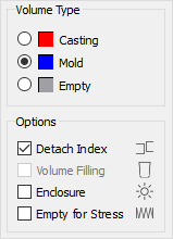
It is necessary to ensure that the mold material density is specified in the Thermal tab of the property editor for the volumes involved in the outgassing calculation (see the figure below). This means that the specific heat capacity is entered in combination with the density, rather than just the volumetric heat capacity. Density is required as a parameter for calculating the initial (i.e., before the onset of thermal destruction) specific mass of the binder in the mixture. Specifying the density as a constant value will directly apply to this calculation. If a density curve is specified, the value corresponding to the minimum specified temperature will be used.
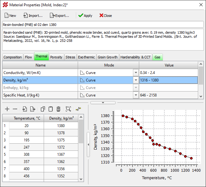
In addition to preparing a geometric model, a lot of data is required for the calculation, such as: thermophysical and mechanical properties of materials and alloys, heat transfer parameters between bodies and with the environment, temperature, speed conditions, etc. Some of this data: material properties and heat transfer parameters, is mandatory for any calculation; others are used depending on the case. Editing, storage and other operations with this data are performed in the same type of editors, a description of which is given below in the relevant sections.
The Project Data tree is a convenient tool for quickly viewing boundary conditions and data assigned in volumes and at the boundaries of the calculation area, as well as a starting point for assigning new conditions. The tree is located on the Project Overview tab (1), which is located on the left side of the Master module (see the figure below).
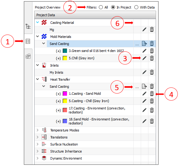
The top of the tab contains filters that can be used to change the amount of information displayed in the tree (2). When loading a project, the In Project filter is automatically set to display only information about the project data in the tree. The volume and boundary indices assigned in the project are indicated in the tree by the "(+)" sign at the beginning of the line.
Each tree position has a button (3), at the end of the line, which launches the corresponding data editor. To delete data for a selected tree line, for example, a material, click the button (4). If this icon is missing, the data has not yet been created.
For many calculation conditions, such as Mold Materials, Heat Transfer, Translations, the data can be loaded from previously saved files, or, conversely, exported, in order to use them in other projects. To export data for all conditions, use the button , located in the data set line (5), and to import, use the button located there. The POLIGONSOFT database contains ready-made settings for parameters and materials for different casting technologies, which can be loaded into the project in a similar way and, if necessary, edited for a specific task. Some conditions, such as "Casting Material" or "Dynamic Environment" do not have import and export buttons (6), they can only be imported or exported directly from the editor.
The material properties, boundary conditions and other data editors, despite the fundamental differences, have the same interface. The window of any editor contains a toolbar (1), a table of editable parameters (2) and an area for editing curves (3) (see the figure below). If there is a * symbol at the end of the editor's caption, it means that the parameters have been changed. When you close the editor, you will be prompted to save your changes.
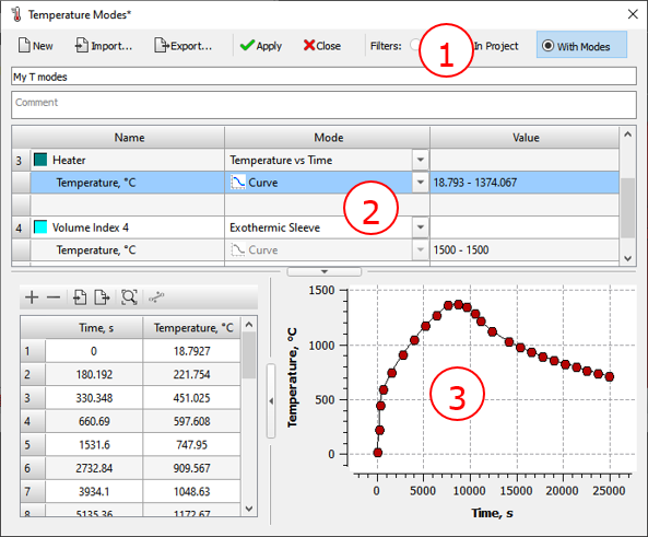
In some editors under the toolbar (1) there is a line where you can enter the name of the data set. This name will then be displayed in the corresponding line in the parameters table (Start Simulation and Parameters window). Below is a line for entering a comment on the data set. In most cases, the dataset name is edited in the tree on the Project Overview tab.
When creating or editing data for a specific volume index, boundary, etc., the editor is launched from the corresponding tree on the Project Overview tab. If the data has not yet been created, all elements of the editor interface are inactive (see the figure below). To start working in the editor, click the New button, which will activate its interface.
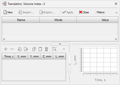
Further in this section, interface elements and buttons common to all editors are considered. The following sections give more detailed descriptions of all editors and the data edited in them.
All editors have a toolbar at the top with buttons for general data operations (see figure below). The number of commands may vary depending on the functionality of the editor.

 |
The New button creates a new data set with "default" parameters. The data is created for use in the current project. |
 |
The Import button opens a standard dialog for loading data into the project. It is possible to import data created in older versions of POLIGONSOFT. |
|
The Export button export data from the project to files that can form a user database and then be used in other projects. This command is also used if you want to save edited data in the original file. |
 |
The Apply button saves the imported or/and edited data in the project. The original data file remains unchanged. To update it, use the Export button. |
 |
The Close button closes the editor. If the data in the editor has been changed, a message will be displayed asking you to save it. |
On the right side of the toolbar are filters that change the set of displayed data:
Many material characteristics and simulation conditions can be specified either by constants or by curves. In this case, the drop-down list is active in the parameters table, in the Mode column (see the figure below).
If Value is selected, then the parameter should be set as a constant in the Value column. If Curve is selected, the curve editing area at the bottom of the editor becomes active. It contains: on the left - a table with coordinates of points and a toolbar for working with a curve; on the right is the curve drawing area (see the figure below).
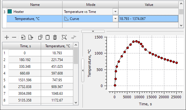
Above the table with the coordinates of the curve points there is a toolbar with buttons that control the data in the table.
 |
The Add Row button creates a new row in the table. The row is created under the current (active) table row. New row cells default values based on the values set in the previous and next cells. At the same time, a new point is displayed in the curve drawing area, it is highlighted in yellow. |
 |
The Delete Row button deletes the selected row in table. |
|
The Import Curve Points button opens a standard dialog for loading data into a table. It is possible to import data from .csv (MS Excel), .lin (POLIGONSOFT) files and any other text files containing curve points in the "x y" format. |
|
The Export Curve Points button exports the data from the table to a .lin text file (POLIGONSOFT) that contains the curve points in the "x y" format. The file can be imported into other spreadsheet editors such as MS Excel. |
 |
The Copy Table button copies the table to the clipboard. The data can be pasted into another table or into another application. |
 |
The Paste Table button pastes data from the clipboard. |
|
The Delete Table button deletes all table rows. To delete one or more selected table rows, use the button. |
Editing the table results in an immediate change in the appearance of the curve in the drawing area on the right. The curve must contain at least two points. The table of editable parameters will display the minimum and maximum values of the parameter.
The drawing area is interactive, the user can change the appearance of the curve and edit it with the mouse.
 |
The Fit button returns the curve display to its default state. |
 |
The Line button allows you to create a linear section of the curve between two selected points. When two points are selected, the button becomes active. On fig. below is an example of how this command works. |
|
|
Initial curve |
Curve with linear section |
Some editors have parameters whose values can not only be set by the user, but also calculated using other set parameters. For example, some characteristics of a casting alloy, necessary for the shrinkage porosity model, can be calculated using other properties, such as density. If a parameter can be calculated, there is a button with a calculator in the right side of the cell where the value is usually entered (see the figure below).
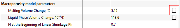
The calculated values can be edited or replaced with other values at the user's discretion. The requirements for the calculated parameters and the calculation methodology are described in the relevant sections.
The Material Properties editor (see figure below) is used for creating and editing materials used in the calculation. Materials are stored in the %POLIGONSOFT%\Database folder in pmat files (older versions have bd, fil and bdd extensions). Each material must contain a set of characteristics required for POLIGONSOFT solvers: Euler, Fourier, Hooke, etc.
|
The button to launch the Material Properties editor is located on the Process toolbar and on the Main tab of the ribbon menu. The editor can also be opened from the Materials tree on the Project Overview tab and from the Start Simulation and Parameters window. See Materials Assignment section for more details. |
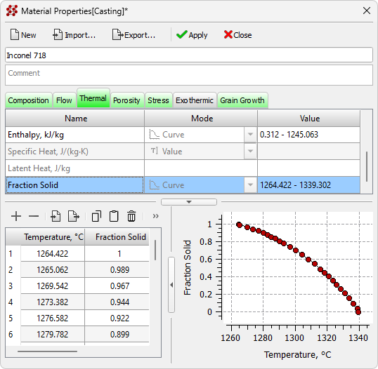
Under the toolbar there is a line with the name of the material, which can be changed. The comment box is located below. The following is a table of material properties, with properties divided into tabs:
Tabs can be of three colors (see the figure below): gray - the tab does not contain data; green - the tab contains the minimum set of material properties that are sufficient to run the solver; pink - the set of properties is not enough to run the solver.
On the tab marked in pink, the properties that are not set but required to run the solver are also highlighted in pink (see the figure below).
The ability to import material properties in a legacy format is retained. Older versions of materials have the extensions bd (thermal properties), fil (shrinkage properties) and bdd (mechanical properties). When importing a bd (thermal properties) file, other file types with the same name are searched. If other alloy properties are found, the Master offers to load them into the appropriate tabs (see the figure below).
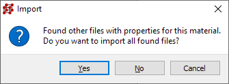
When importing fil (shrinkage properties) and bdd (mechanical properties) files, the properties are loaded into the respective tabs, but other file types are not searched.
The tab contains a table of chemical composition (see figure below). In the first line of the table, you can select the base element of the alloy (Fe, Al, Ni, Ti, etc.) and then enter the content of the remaining elements in weight percent.
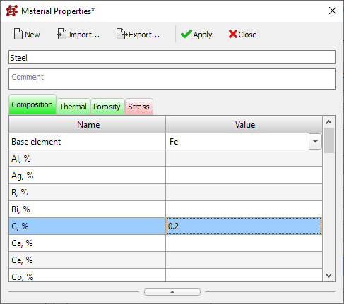
The tab turns green if the content of at least one chemical element or a basic element is specified in the table.
The data in this tab can be used as input for the Heat Treatment solver (for more details see the Heat Treatment Simulation) section).
The tab contains material characteristics related to its behavior in the liquid state (see figure below).
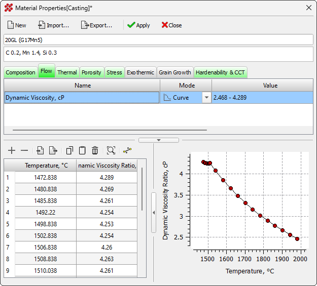
Dynamic Viscosity is required for the continuous casting hot tearing model. It can also be used to calculate the Kinematic Melt Viscosity parameter, which is used to model microporosity (see the Porosity Tab for more details).
The tab contains a set of material characteristics required to calculate the temperature and phase fields (see the figure below). To calculate temperature fields in bodies where there is no phase transition (usually it is a mold), the minimum set of thermophysical properties required for calculation includes:
These properties can be specified either as constants or as functions of temperature.
In the presence of a phase transition, i.e. solidification (usually these are bodies of the “casting” type), you should additionally specify the following characteristics:
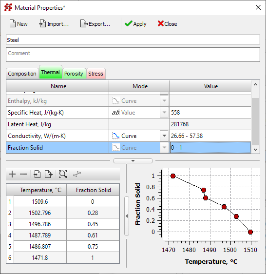
The Solid Fraction is a function of temperature. Its values should start from 0 at the liquidus temperature and increase to 1 at the solidus temperature. Thus, the fraction of the solid phase is determined by a falling curve strictly between 0.0 and 1.0. Isothermal transformation (for example, eutectic) is recommended to be "stretched" by an interval, for example, of 2-3 degrees. Latent Heat is given by a constant.
It should be noted that the POLIGONSOFT algorithms allow you to set the fraction of the solid phase with flat sections. The recommendation to "stretch" them by 2-3 degrees is not mandatory.
An alternative way of defining the phase transition is possible. Instead of Specific Heat and Latent Heat, the corresponding Enthalpy curve can be given as a function of temperature H(T), which is defined as follows:
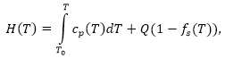
Since there are two ways for defining a phase transition, the editor automatically avoids conflict between the following options:
or
If specific heat or latent heat is entered, the enthalpy entry is blocked, and vice versa.
Thermal conductivity and enthalpy must always be given as a temperature curve.
The tab contains a set of material properties needed to calculate pipe shrinkage, macro- and microporosity in a casting (see the figure below).
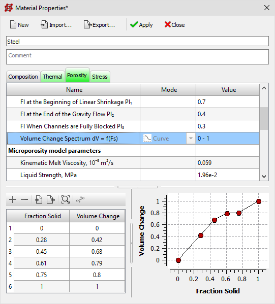
The set of parameters required for the "standard" macroporosity model used in POLIGONSOFT:
Some parameters can be calculated based on the properties specified in the Thermal tab. This mainly requires the Density specified as a function of temperature and the Fraction Solid curve. The calculated values can be edited or replaced with other values at the user's request.
To calculate the parameter, you should click the calculator button in the right side of the cell (see the figure below).

Melting Volume Change β, %. The parameter, better known as “volume shrinkage”, is calculated using the equation:
In this case, the density values in the liquid and solid state are automatically calculated using the specified density curve at the solidus and liquidus points. If the required temperature values are not among the points of the density curve, they will be found using the linear interpolation method for the neighboring points. This approach is used when calculating all other parameters.
Liquid Phase Volume Change βL, 10-6/K. The parameter is the coefficient of thermal linear expansion of the liquid phase above the liquidus temperature Tliq. It is calculated using two points of the density curve: one point, for example, is the last point of the curve at the maximum temperature Tmax, the second point is the density at Tliq:
Volume Change Spectrum dV(fs). The curve characterizes the change in volume during the solidification process. The horizontal axis shows the values of the Fraction Solid, specified by the fs(T) curve on the Thermal tab. The vertical axis shows the corresponding Volume Change, calculated using the equation:
It is easy to see that when fs = 0 the density ρfs = ρliq and dV = 0, and when fs = 1 the density ρfs = ρsol and dV = 1.
To calculate microporosity according to the "standard" POLIGONSOFT model, in addition to the parameters listed above, it is required to set the parameters:
To calculate the filtration coefficient using the equation:
| where |  |
need to define:
Kinematic Melt Viscosityγ, 10-5 m2/s can be calculated if the dynamic viscosity curve is specified in the Flow tab and the density curve in the Thermal tab. The parameter characterizes the melt flow in the two-phase region near the solidus temperature and is calculated using the equation:
To calculate the parameter, you should click the calculator button in the right side of the cell.
At the end of the table, the set of parameters required for the new porosity model is listed, which extends the capabilities of the "standard" macro- and microporosity models:
Some parameters from this list duplicate the parameters of the "standard" macroporosity, but nevertheless must be set again. This is because the parameter values are different when used in different models and their separation is convenient for switching between new and standard porosity models.
For more information on the new model of porosity and its parameters, see the New Pipe Shrinkage and Macroporosity Model section.
The tab contains a set of material properties required to calculate the stress-strain state of the casting and the mold (see the figure below).
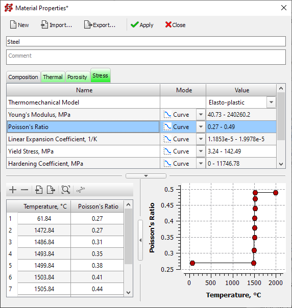
Different stress models can be used in the calculation, each requires its own set of mechanical characteristics. The stress model is selected from the list, which is located in the first line of the parameter table. The following options are available:
The Linear Elastic model is characterized mainly by Young's Modulus. In addition, the Poisson's Ratio and the Thermal Expansion Coefficient must also be specified. The value of Poisson's Ratio for metals is approximately 0.3.
For an Elasto-plastic model, the properties described above for an elastic model, i.e. Young's Modulus, Poisson's Ratio and Thermal Expansion Coefficient must also be given. In addition to this, the Yield stress and Hardening Coefficient must be specified. Hardening Coefficient, as a first approximation, can be calculated using a simple formula:
H(T) = E(T) / 20,
To calculate the parameter, you should click the calculator button in the right side of the cell.
All listed properties can be specified by constants or temperature curves. Of course, it is extremely undesirable to set the properties with a constant, since in this case the accuracy of the calculation decreases. For example, if all properties are given by constants, then the result of the calculation will in no way depend on the change in the temperature field of the casting and the mold.
The source of stress properties can be: literature, the Internet and scientific research. If these sources cannot provide the necessary data, then they can be obtained empirically, i.e. by carrying out the necessary mechanical tests.
The tab contains a set of parameters (see the figure below) necessary for heat release simulation when using mold elements made of exothermic (thermitic) mixtures (sleeves, covers, mats, etc.). Such a material must be specified in the model as a separate volume of the “mold” type with the necessary thermophysical properties are specified on the Thermal tab (for more details see the Thermal Tab section). Then the required parameters for the exothermic reaction should be specified:
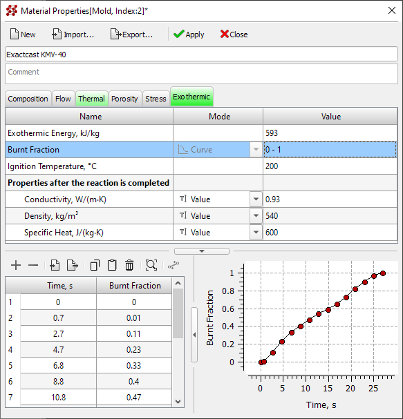
If at least one of the three parameters described above is not set, the tab will be colored pink. This means that there is not enough data to run the calculation. The corresponding parameter lines will also be pink. If all parameters are set, the tab is colored green.
Additionally (but not necessarily) the thermophysical properties of the material after completion of the reaction can be specified. They differ from the initial exothermic material properties, specified on the Thermal tab, and can be used in the calculation to take into account the heat-insulating ability of burnt material. The following properties will be used when calculating temperatures for those mesh nodes where the burnt fraction is equal to 1:
These properties can be specified by constants, or temperature curves. All three properties must be set. If the properties of the material after the completion of the reaction are not set, then properties from the Thermal tab will be used for the heat transfer calculation in the areas, where the fraction of burnt material is equal to 1.
When using exothermic materials, it may be necessary to enter specific heat transfer parameters at the casting-material and material-mould interfaces. These parameters are set in the Heat Transfer editor (see the Heat Transfer Parameters section). For more information on modeling foundry technology using exothermic materials, see the Exothermic Sleeves section.
The tab contains coefficients determined by the chemical composition of the alloy, which are used in the equation for the growth rate of the primary axis of the dendrite in the grain growth model (see figure below). This data is used by the Macrostructure solver. For more information about macrostructure simulation, see the Macrostructure Simulation section.
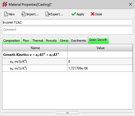
The tab contains the data required to calculate the microstructure and properties in the model bodies of the "casting" type, using the following models:
For more information on modeling heat treatment processes using different models, including those listed above, see the Heat Treatment Simulation section.
For calculations using the model based on hardenability, it is necessary to specify data characterizing the conditions and results of standard (EN ISO 642) tests for hardenability (see the figure below):
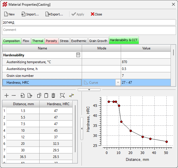
For calculations using GPBM, it is necessary to enter the thermokinetic diagram (CCT) of austenite decomposition during continuous cooling and the conditions for obtaining it (see the figure below). The conditions in which the CCT was obtained are described by the following parameters:
The sum of the proportions of ferrite and pearlite under equilibrium conditions should be 100%.
To draw the CCT diagram, a separate data entry will be required for each of its branches in the form of pairs of values “cooling rate in °C/s – transformation temperature in °C”.
When entering data to draw the CCT diagram, the following rules should be followed:
Input control can be performed using the diagram constantly displayed at the bottom (see the figure below). For convenience, branches on the diagram are also plotted in the coordinates "cooling rate - temperature" (default display type of CCT diagram in the editor window).
Usually, the curves of the beginning and end of the transformation (except for martensitic) are convex upwards. This corresponds to the fact that the lower the cooling rate, the higher the temperature of the beginning or end of the transformation. This allows the most correct transformation of the CCT diagram into an isothermal decomposition diagram (TTT) and the description of the family of C-shaped curves by Zener-Hillert dependencies.
The input of the curve of the end of the ferrite transformation is not provided, since it coincides with the curve of the beginning of the pearlite transformation.
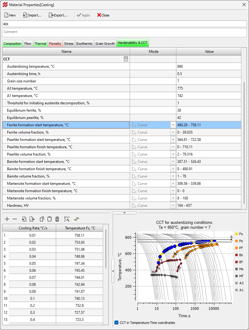
To display the CCT diagram in the form familiar to a thermal engineer in the “temperature-time” coordinates, you should check the CCT in Temperature-Time coordinates checkbox, it is located under the diagram.
The hardenability curve and thermokinetic diagram can be calculated. To access the corresponding generator (see the figure below), click the calculator button in the parameter group name line. Calculations are based on the steel's chemical composition and austenite grain size, which can also be calculated based on the austenitizing temperature and time. The data obtained in this way can be used in heat treatment process analysis using the hardenability-based model and GPBM, and are also generally useful for designing heat treatment modes. For more information on performing calculations, see the Heat Treatment Simulation section.
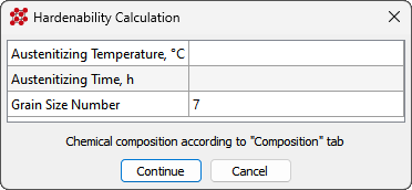 |
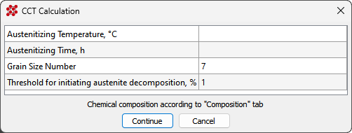 |
a) |
b) |
The hardenability curve is calculated using the Grossman method [1], modified to take into account the austenite grain size. The result of the calculation is a hardenability curve in the coordinates "distance from the hardened end of the sample" (mm) – "hardness" (HRC), which is obtained in practice during standard testing.
The CCT calculation is based on the initial calculation of the TTT diagram using the metod [2] followed by its transformation into the CCT using the Sheil additivity rule [3]. A series of other models were also used in the complex calculation:
The result of the CCT calculation is a series of cooling rates and the corresponding temperatures of the beginning and end of the transformations of ferrite, pearlite, the temperature of the beginning of the transformation of martensite, bainite (if the transformation occurs at a given speed), the volume fractions of ferrite, pearlite, bainite, martensite (if the transformation occurs) and hardness.
Generators can only be used to calculate the properties of hypoeutectoid steels. Chemical composition restrictions are listed in the table below.
| Table. Permissible limits for chemical element content when using generators. |
| Element | Content limits, % | |
| Basic elements | ||
| C | 0.05-0.60 | |
| Si | ≤1.37 | |
| Mn | ≤2.00 | |
| Cr | ≤3.00 | |
| Ni | ≤4.00 | |
| Mo | ≤1.00 | |
| Residual levels | ||
| Cu | ≤0.15 | |
| Al | ≤0.06 | |
| Nb | ≤0.02 | |
| V | ≤0.20 | |
| Ti | ≤0.20 | |
| W | ≤0.20 | |
| B | ≤0.0008 | |
| N | ≤0.012 | |
| Co | ≤0.10 | |
| Mg | ≤0.005 | |
| Sn | ≤0.01 | |
| Zr | ≤0.005 | |
| S | ≤0.035 | |
| P | ≤0.035 | |
After launching the hardenability or CCT generator, you must assign the initial data for the calculation in its window. After the generator completes, the calculation results will be saved in the corresponding section (Hardenability or CCT) of the editor. The calculations are performed independently: only hardenability, only CCT, or both can be generated.
To obtain the result, you should act in the following order.
| Table. Restrictions on the input of initial data for generating hardenability and CCT |
| Parameter | Range |
Austenitizing Temperature, °C |
750 - 1200 |
Austenitizing Time, h |
0.1 - 5 |
Grain Size Number |
-7 17 |
Threshold for initial austenite decomposition |
0.1 - 1 |
The Gas tab contains a set of properties (see the figure below) necessary for modeling the mold's gas regime. The parameters on this tab are divided into two groups. The properties in the Filtration Properties of Compacted Sand Mixture group are needed to calculate the transport of gases driven by pressure differences due to uneven temperature distribution within the mold and gas formation during binder gasification. Gasification parameters are specified in the Gas Evolution Due to Binder Decomposition group. If no characteristics are entered in the second group, the material will be considered non-gassy. The movement of gases in a non-gassy form is determined solely by their thermal expansion within the pores during mixture heating.
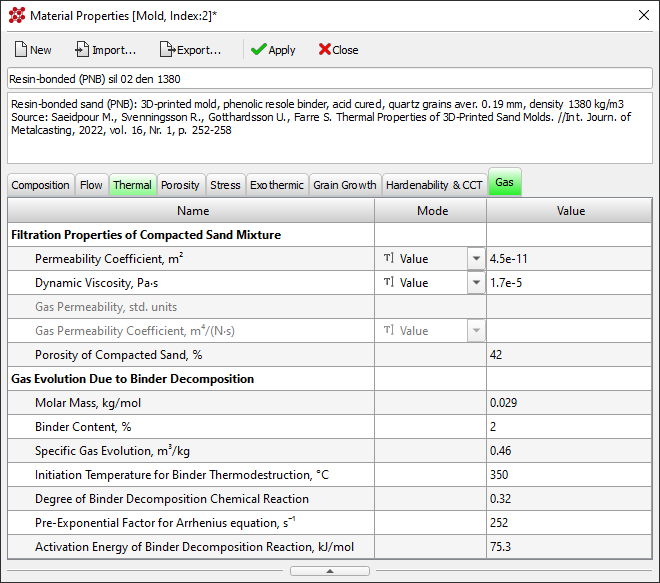
In the Filtration Properties of Compacted Sand Mixture group the following properties are specified.
Depending on the available data, the following combinations of parameters can be entered:
or:
or:
In the Gas Evolution Due to Binder Decomposition group the following properties are specified.
The Heat Transfer editor is designed to create and edit heat transfer settings at the boundaries between volumes (Body-to-Body) and at the outer boundaries (Body-Environment). The settings can be applied to solve one specific problem or exported to a file with the afo extension for use in other calculations, including as a casting process template.
|
The button to launch the Heat Transfer editor is located on the Process toolbar and on the Main tab of the ribbon menu. The editor can also be opened from the Start Simulation and Parameters window and from the Heat Transfer tree on the Project Overview tab. |
In the editor table, heat exchange conditions are specified for all surfaces of each volume of the computational domain. Heat exchange parameters for each surface (boundary) are determined by a specific task and depend on where this boundary is located. The list of boundaries does not include a boundary with index 0, since this boundary is either internal or external with adiabatic conditions and no parameters need to be specified for it. To display in the table only those boundaries that are specified in the model, you can use the In Project filter located on the toolbar (see the figure below). To display a list of boundaries where data is specified (not all boundaries may be present in the project), use the With Data filter. The Current filter shows only the boundary selected in the tree on the Project Overview tab.
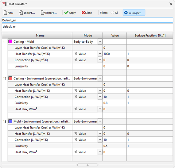
The list of heat transfer parameters for each boundary begins with a line that specifies its index and color, which is used for visualization in the pre- and postprocessor in the boundary indices mode. In the same line, in the Name column, you can enter an explanatory text describing, for example, the heat transfer conditions. This text will be displayed in preprocessor dialogs when editing boundaries. The next column Mode indicates one of the two heat transfer modes. For boundaries with indices 1-9, it can be changed. Сlicking on a line brings up a drop-down list in which you need to select the desired option (see the figure below):
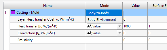
As indicated in the Basic concepts: Volumes, Types, indices section, the first nine boundaries, starting from index 1, are universal and can be used as boundaries between bodies of the computational domain or as external boundaries with the environment. All other boundaries with indices 10-18 set the parameters of heat transfer between the body and the environment.
In the Body-Environment boundary mode, the Ambient Temperature line becomes available.The ambient temperature can be set by a constant value or by a time-temperature curve. To select, you need to click the left mouse button in the Mode column and select the desired option from the drop-down list (see the figure below).
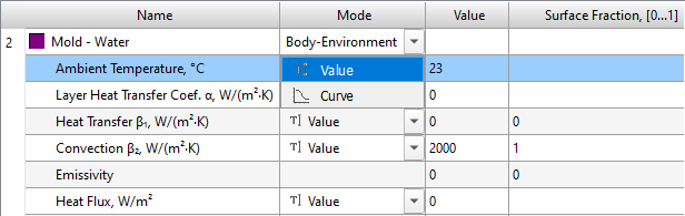
If the ambient temperature is constant, select the Value mode and set the temperature in the next cell Value. If the ambient temperature changes depending on time, select the Curve mode. In this case, the table and the curve drawing area in the lower part of the editor window become active, where you can set the points of the curve in the time-temperature coordinates (see the figure below). For more information on editing curves, see the Editing Constants and Functions section.
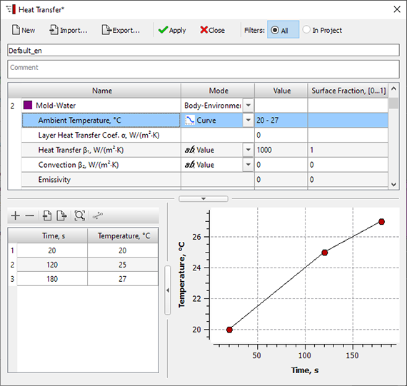
It should be note in mind that for boundaries 17 and 18, the ambient temperature is set by a constant in the Start Simulation and Parameters window.
The next four lines set the heat transfer parameters, in accordance with the POLIGONSOFT model . This model can be represented as a scheme (see figure below) and describes three mechanisms of heat transfer: heat conduction, convection and radiation.
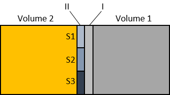
It is assumed that, in the general case, at the boundary between volume 1 and volume 2, two successive layers can exist: let us designate them as I and II. Layer I is characterized by the heat transfer coefficient of the layer α, which is set by the user. For example, this could be a coating applied to a mold. If the thermal conductivity of the coating material λI and its thickness δ are known, then the heat transfer coefficient of the layer α can be calculated by the equation:
 |
(1) |
Layer II is characterized by a calculated heat transfer coefficient β. In general, the contact between volumes 1 and 2 is not ideal. It is assumed that heat transfer in layer II can take place in three ways: heat transfer in the zone of direct contact of volumes, convection and radiation where there is no contact. Each mechanism acts on a part of the boundary, which is specified by the relative areas S1, S2 and S3 respectively. Thermal conductivity and convection are given by the heat transfer coefficients (let's call them β1 and β2). The radiation is characterized by a given emissivity E. Then the calculated heat transfer coefficient β can be calculated as:
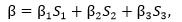 |
(2) |
where |
Knowing the coefficients α and β, one can write down the equation for a heat flux density:
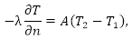 |
(3) |
where |
At the outer boundaries of volumes, heat transfer in the general case can be carried out by heat transfer, convection and radiation. In addition, a constant heat flux can be specified at the outer boundary. The heat flux density in general is determined by the expression:
|
(4) |
where q – heat flux; |
Using the described model, the user can specify any mechanism for transferring heat from body to body or from body to environment. The following lines are used for this:
To switch off one or two heat transfer mechanisms from the calculation, it is necessary to set the corresponding fraction of the surface equal to 0. At least one of the three mechanisms of the second layer must be enabled.
Data from files of outdated formats that were used in previous versions of POLIGONSOFT can be imported into the project:
Temperature Modes editor is intended for creating and editing temperature modes of the casting and mold volumes. The settings can be applied to solve one specific problem or exported to a file with the .tel extension for use in other calculations. The ".tel" temperature file can be a part of a casting process template.
|
The button to launch the Temperature Modes editor is located on the Process toolbar and on the Main tab of the ribbon menu. The editor can also be opened from the Start Simulation and Parameters window. |
In the table that occupies the upper part of the editor (see the figure below), temperature modes are set for all volumes of the model, for which you need to set special conditions that differ from those specified in the Start Simulation and Parameters window on the General tab (see deatils in Сommon Simulation Parameters section). Regardless of the problem being solved, the table always contains data on all 9 volume indices, which in general can all be specified in the model (more details about volume indices see in Basic concepts: Volumes, Types, Indices section). To display in the table only those volume indices that are specified in the model, you can use the In Project filter located on the toolbar (see the figure below). To display only volume indices with specified temperature modes, use the With Modes filter. Use the All filter to display the entire list of volume indices.
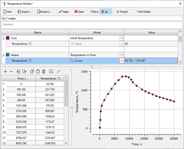
For each volume index, the Name column contains the index, its color designation and explanatory text (name of the volume). In the next column Mode there is a switch for the set temperature mode. From the drop-down list it is proposed to select:
Please note that the temperature set for the volume index will be applied to all volumes with this index regardless of their type (casting or mold). Pay attention to the temperature icons in the Model Tree to avoid mistakes.
The selected temperature mode is set in the Temperature line. This line is visible only if the temperature mode is set for the volume index. In the Initial Temperature mode, the temperature can only be set by a constant in the Value column. In the Temperature vs Time with Cutoff mode, the temperature can only be set by the curve in temperature-time coordinates.
If the Temperature vs Time mode is set, in the Mode column you can select one of the options: Value or Curve. If Value is selected, the temperature of the volume(s) of the selected index is set by a constant in the Value column. This means that the temperature in the volume(s) will be constant throughout the entire calculation
If the Curve option is selected, the table and the curve drawing area become active at the bottom of the editor, where you can specify the points of the curve in temperature-time coordinates. If the calculation time exceeds the time set for the last point of the curve, the temperature of the volume(s) remains equal to the temperature set for the last point of the curve. For more information on editing graphs, see the Editing Constants and Functions section.
For the procedure for saving temperature modes and descriptions of other buttons located on the panel, see Toolbar Buttons section.
The Dynamic Environment editor is designed to create and edit an environment consisting of several layers with changing parameters. The settings can be applied to solve one specific problem or exported to a file with the pdes extension for use in other calculations (import of older files with the air extension is also supported).
|
The button for launching the Dynamic Environment editor is located on the Process toolbar and on the Main tab of the ribbon menu. The editor can also be opened from the Start Simulation and Parameters window and from the tree on the Project Overview tab. |
The dynamic environment is an environment that is divided vertically into 5 layers. Each layer has its own characteristics (height, temperature, and other parameters described below), some of which can change during the simulation. These settings overlap the parameters of the "normal" environment, which are set in the Start Simulation and Parameters window on the General tab (for more details, see the Сommon Simulation Parameters section) and in the Heat Transfer editor (for more details, see the Heat Transfer Parameters section). The dimensions of each layer are determined only by its height or thickness; in the other two directions, the layer is infinite.
During the calculation process, the casting and mold can be stationary in one or more layers simultaneously, can move through these layers and go beyond them. Outside the dynamic environment, normal environmental conditions apply.
In the table that occupies the upper part of the editor (see the figure below), the parameters of the layers of the dynamic environment are specified, for which it is necessary to set special conditions that differ from those specified in the "Parameters and run calculation" window on the "General" tab (for more information, see the Сommon Simulation Parameters section). Regardless of the problem being solved, the table always contains data on all 5 layers of the environment, but some layers can be switched off and thus the dynamic environment will have gaps where heat exchange will proceed according to the rules of the "normal" environment.
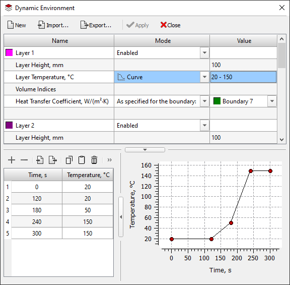
For each layer, the Name column by default indicates its name, number and color designation (the name can be replaced with a custom one). The next column, Mode, contains the layer activity switch. From the drop-down list, you can select:
Below are the layer parameters:
It should be remembered that even if the dynamic environment layer is disabled, its height matters, since it sets the gap between adjacent layers or an additional layer of "normal" environment on the edge.
For information on the procedure for importing/exporting a dynamic environment and a description of other buttons located on the toolbar, see the Toolbar Buttons section.
When modeling some foundry processes, it is necessary to take into account the movement of casting and/or mold volumes. For example, when simulating vacuum casting, you may need to take into account the movement of the mold within the furnace. To create and edit volume movements, use the Translation editor and the Translations tree in the Project Overview panel. Translation modes can be configured and used to solve one specific problem, or imported (and exported) into the project from files with the pmov extension (importing files of older versions with the mve extension is also supported).
|
The Translation editor button is located on the Process toolbar and on the Main tab of the ribbon menu. The editor can also be opened from the Translation tree on the Project Overview tab. |
The editor title indicates the volume index the translation mode will be created for, for example, in Fig. Below is the editor for moving volumes with index 2. Please keep in mind that the specified mode will be applied to all volumes with index 2, regardless of their type (casting or mold). If the translation mode has not yet been specified, then all interface elements are inactive. To start working in the editor, you need to create a translation mode for the selected index - click the New button.
Unlike other editors, there are no Import and Export commands on the toolbar, since these operations are performed through the Translations tree (for more details, see the Project Overview Tab section). Otherwise, the principles of operation follow the general rules described in Data Editors. General Controls and Features and Editing Constants and Functions sections.
The translation mode for the selected volume index is set by the table at the bottom of the window (see the figure below). For each line, the first column Time indicates the moment in time, the next three columns indicate the shift in x, y, z coordinates relative to the previous position described in the previous line. The fourth column “L” is not editable, it shows the shift value, which is calculated using the equation:
|
where Xt, Yt, Zt – shift coordinates at time t; |
The L(t) graph is displayed to the right of the coordinate table.
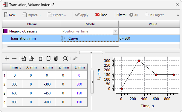
Unlike most other editors, here you can set a single-point movement schedule. In this case, bodies with the specified index will be instantly moved in the specified direction. This can be useful for modeling processes that do not require the action to be performed in time, such as opening a mold in high-pressure casting.
Often, translation is used when simulating vacuum casting in combination with radiation heat transfer (for more details, see the Radiation Heat Transfer section). Often, translation is used when simulating vacuum casting in combination with radiation heat transfer (for more details, see the “Radiation Heat Transfer” section). If translations are specified, a ray tracing calculation will be performed for each point in the graph, and linear interpolation between two adjacent times for all intermediate points in time will be used. For such calculations, you should specify the number of points necessary for a qualitative description of the visibility of objects during the entire calculation. But it should be remembered that a large number of points in the translation curve significantly slows down the calculation with radiation heat transfer.
All specified translation are displayed in the Translations tree on the Project Overview panel. They can be exported to a .pmov (for more details, see the Project Overview Tab section). This file can then be imported into another project (importing files of older versions with the mve extension is also supported).
For some castings, requirements may be imposed on the quality of the macrostructure: size, shape, quantity and orientation of grains. POLIGONSOFT allows you to model the processes associated with the nucleation and growth of the grain structure of the metal (for more details, see the Macrostructure Simulation section). To create and edit boundary conditions describing the process of grain nucleation at the casting-mold boundaries, use the Surface Nucleation editor and the tree of the same name in the Project Overview panel. Nucleation conditions can be configured and used to solve one specific problem, or imported (and exported) into the project from files with the psn extension.
|
The button to launch the Surface Nucleation editor is located on the Process toolbar and on the Main tab of the ribbon menu. The editor can also be opened from the Surface Inception tree on the Project Overview tab. |
The editor header indicates the index of the boundary for which the generation parameters will be created, for example, in the figure below the editor is open for the boundary with index 1. If the parameters have not yet been set, the editor looks like in the figure below, all interface elements are inactive. To start working in the editor, you need to create generation parameters for the selected boundary - click the Create button.
Unlike other editors, there are no Import and Export commands on the toolbar, since these operations are performed via the Surface Nucleation tree (for more details, see the Project Overview Tab section). Otherwise, the operating principles follow the general rules described in the Data Editors. General Controls and Features and Editing Constants and Functions sections.
The parameters for the grain structure generation for the selected boundary index are specified in the table (see the figure below). In the first line of the editor, you can enter a name for the data set being created. By default, the boundary identifier is used.
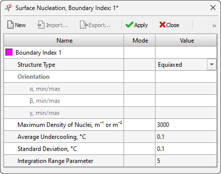
The appearance of solid phase nuclei in a supercooled melt is a random process. The number of nuclei that appear in the melt when the supercooling changes by a small d(ΔT) value is described by the Gaussian distribution (see equation (3) in the Grain Nucleation Model section). The nucleation of the solid phase for the casting-mold boundaries is determined by the following parameters:
Macrostructure simulation (for more details, see the Macrostructure Simulation section) can be performed either in the entire casting or in a certain specified area, which is set in the Start Simulation and Parameters window on the Structure tab (for more details, see the Macrostructure Simulation Parameters section). To obtain results corresponding to the specified technology, it may be necessary to set the conditions for inheriting the structure on the faces of the parallelepiped that limits the calculation area.
For example, the figure below shows the structure modeling area, in which the structure will be generated on the side faces in accordance with the surface nucleation conditions at the casting-mold boundary. In this case, the upper and lower faces of the area border on the melt, where the nucleation conditions cannot be specified, since there is no boundary. To take into account the influence of the structure formed outside the calculation area, it is possible to apply the mechanism of its inheritance from neighboring areas of the casting.
To do this, use the Structure Inheritance editor and the tree of the same name in the Project Overview panel. The inheritance conditions can be configured and used within the framework of solving one specific problem, or imported (and exported) into the project from files with the pinh extension.
|
The button for launching the Structure Inheritance editor is located on the Process toolbar and on the Main tab of the ribbon menu. The editor can also be opened from the Structure Inheritance tree on the Project Overview tab. |
The Structure Inheritance tree contains 6 lines corresponding to the six faces of the parallelepiped that limits the calculation area. Since the faces of the parallelepiped are parallel to the coordinate planes, they are designated by icons with filled faces. The face color corresponds to the color of the axis perpendicular to which the face is located. When calling the editor, the face is identified in its header by the axis and position relative to the origin: Xmin, Xmax, Ymin, Ymax, Zmin and Zmax. If the parameters have not yet been set, all interface elements are inactive. To start working in the editor, you need to create inheritance parameters for the selected face - click the Create button.
Unlike other editors, the Import and Export commands, as well as filters, are inactive here, since these operations are performed via the Surface Nucleation tree (for more details, see the Project Overview Tab section). Otherwise, the operating principles follow the general rules described in the Data Editors. General Controls and Features and Editing Constants and Functions sections.
The parameters of grain structure inheritance for the selected face of the parallelepiped that limits the modeling area are specified in the table (see the figure below). In the first line of the editor, you can enter a name for the data set being created. By default, the plane identifier is used (for example, Xmin Plane in the figure below).
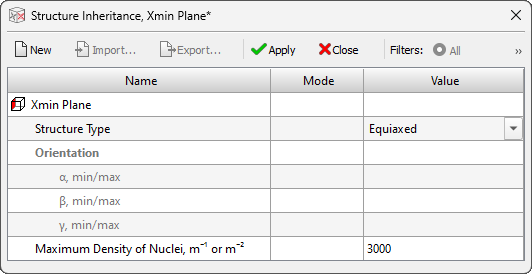
The appearance of solid phase nuclei in a supercooled melt is a random process. The number of nuclei that appear in the melt when the supercooling changes by a small d(ΔT) value is described by the Gaussian distribution (see equation (3) in the Grain Nucleation Model section). The nucleation of the solid phase for the casting-mold boundaries is determined by the following parameters:


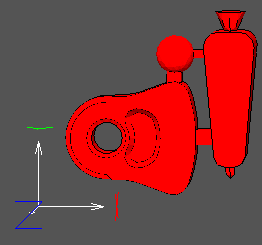
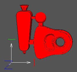
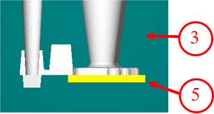
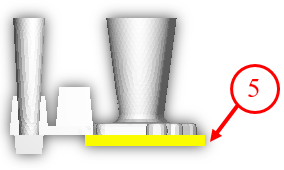
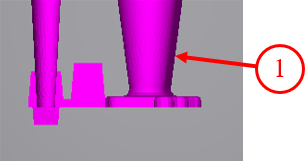
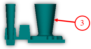
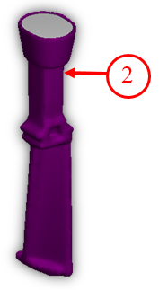
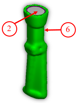
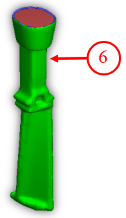
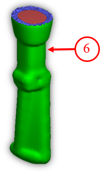
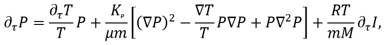
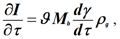
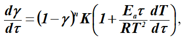
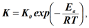
 – radiation heat transfer coefficient.
 .
.
 ,
,.svg)
.svg)
.svg)

.svg)