Modeling of the physical phenomena occurring in the casting and mold is performed by the solver modules of the POLIGONSOFT (see the figure below).
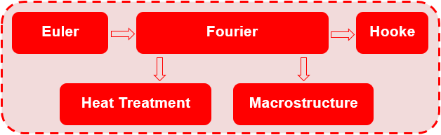
Each solver is responsible for modeling certain physical processes and calculating the fields of the corresponding quantities:
The user can combine solvers to simulate a specific casting technology and obtain the required process information: Euler-Fourier, Fourier-Hooke, or Euler-Fourier-Hooke. Of course, each solver can be run separately from other solvers, provided that all the necessary data is available to run it. The user can also run the same task in parts, for example, at one time to simulate the filling of a mold with a melt (Euler solver), at another time to continue the simulation by running the solidification and porosity calculation (Fourier solver) and then separately calculate the stresses (solver "Hooke"). The transfer of all necessary data from the solver to the solver will be carried out automatically, provided that the name of the project (g3d geometry file) is unchanged. Those. the user can open a project at different times, turn on the desired model (solver), turn off unnecessary ones and perform modeling of the selected process.
To launch each solver, a prepared geometric (finite element) model and a set of parameters describing the properties of the materials used, heat transfer parameters, initial temperature conditions, and other technology parameters are required. The preparation of the geometric model is described in Chapter 5, this chapter discusses the rest of the parameters required to start the calculation.
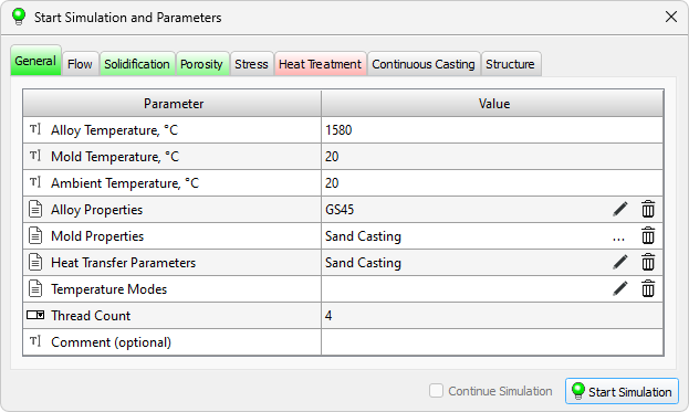
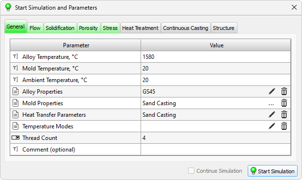
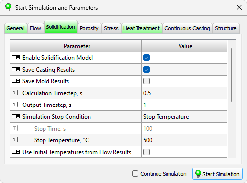
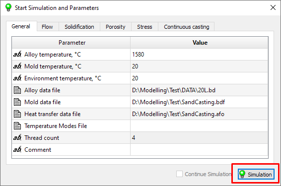
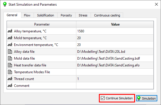
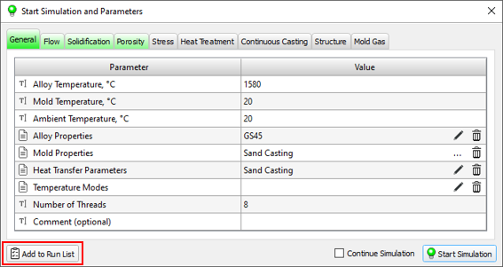
The calculation is started in the Master preprocessor, in the Start Simulation and Parameters dialog. The window contains a table with the parameters required to start the calculation. The options are sorted into the Flow, Solidification, etc. tabs according to belonging to a particular solver. The General tab contains parameters that are required by all solvers.
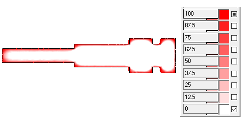
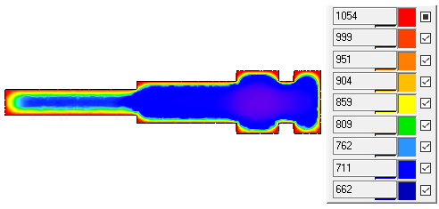
The tabs can be painted in different colors (see the figure below): gray – the model (solver) is disabled; green – the model (solver) is enabled, all the necessary data is specified; yellow – the model (solver) is enabled, all necessary data is specified, but some of them require user attention; red – the model (solver) is enabled, but there is not enough data to run, or it contains errors.
On the tab marked in red, the parameters that are not set but are required to run the calculation or contain errors are also highlighted in red. If a parameter that is required to run the calculation is set but its value is outside the recommended range, it is highlighted in yellow (see the figure above). When you hover the mouse pointer over a yellow or red line, an explanatory tooltip is displayed. The presence of red lines makes it impossible to run the calculation. If there are yellow lines, the calculation can be run, but warnings will be displayed that require user confirmation.
Table on each tab consists of two columns: the Parameter column describes the meaning of the parameter being set, the Value column contains its value. Calculation parameters are specified by different data types, therefore, in each table row, before the parameter name, there is an icon indicating how the parameter is specified. The data types used are listed in the table below.
 |
Checkbox. The parameter can be turned on or off by checking the box in the "Value" cell. |
 |
Switch. The parameter can be selected from the list. To change the parameter, double-click in the corresponding cell of the table and select a value from the list. Editing of a parameter is completed by clicking in any area of the screen. To cancel editing a parameter, press the Esc key. |
 |
Constant. The parameter value is specified as an integer or decimal number, or as a text string. To enter a parameter, double-click in the corresponding cell of the table in the Value column, as a result of which the field will become available for editing. Editing of a parameter is completed either by pressing the Enter key on the keyboard, or by clicking the mouse in any area of the screen. To cancel editing a parameter, press the Esc key. |
 |
File. The parameter value is specified by the full name of the file (including the path), which contains the data required for the calculation. To enter a parameter, double-click in the corresponding cell of the table in the Value column, as a result of which the field will become available for editing. The full file name can be set manually, or by using the button  that will become available at the end of the line when the field is activated. Clicking on this button opens a standard file download dialog. that will become available at the end of the line when the field is activated. Clicking on this button opens a standard file download dialog.When entering the file name manually, you can cancel the editing of the parameter by pressing the Esc key. Some files can be opened for editing directly from the design table. In this case, after double-clicking on the cell, the Edit button  becomes available. Clicking on this button the file opens for editing in the appropriate editor. If you press the Edit button when there is no file name in the cell, the editor will be opened in the mode of creating a new file, which will become the parameter value after saving. becomes available. Clicking on this button the file opens for editing in the appropriate editor. If you press the Edit button when there is no file name in the cell, the editor will be opened in the mode of creating a new file, which will become the parameter value after saving.To delete an attached file, click the  button at the end of the line. button at the end of the line. |
The sections below describe the parameters required to run the different solvers.
The General tab (see figure below) contains the parameters necessary to run the Euler (flow and mold filling) and Fourier (solidification and porosity) solvers. Other solvers don't use this data directly, but they require the Fourier solver to run first. Let's consider the parameters of the tab.
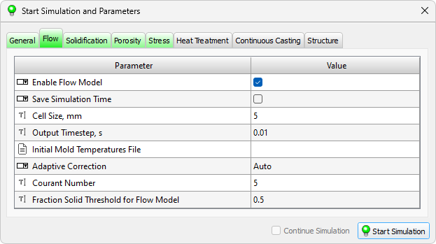
Modeling of mold filling with a melt and other flow cases are performed by the Euler solver. It is designed for coupled hydrodynamic and thermal calculations.
Performing the calculation, the Euler solver following files are written:
In the result of the simulation, the user is given the opportunity to analyze the process of filling the mold with the liquid metal, as well as (and most importantly) to obtain the temperature fields in the casting and the mold at the end of filling, which can be used as the initial conditions for calculation in the Fourier solver, that in some cases significantly increases the reliability of the results.
The parameters required to run the solver are located on the Flow tab (see the figure below).
Casting solidification and cooling simulation, taking into account heat exchange with mold elements and the environment, as well as the prediction of the formation of shrinkage pipes, macro- and microporosity, is performed by the Fourier solver.
In the process of the Fourier solver operation, the following files are written:
In the result of the simulation, the user is given an opportunity to analyze the process of solidification and cooling of the casting, changes in the temperature in the mold, formation of shrinkage defects.
The parameters used to solve the temperature problem in the casting and mold, as well as the problem of solidification of the casting, are located on the Solidification tab (see the figure below).
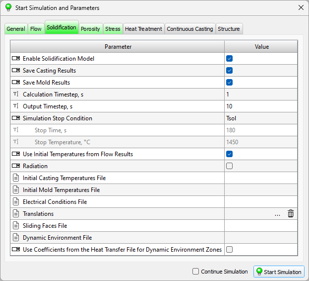
The following calculation parameters are used to set special, additional conditions for calculating solidification.
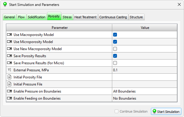
In order to simulate the formation of pipe shrinkage and porosity, in addition to thermophysical parameters (see the previous section), additional parameters should be set. The calculation of porosity and pipes is carried out together with the calculation of solidification, it cannot be performed separately. The parameters used for calculating pipes, macro- and microporosity are located on the Porosity tab (see the figure below).
The separation of the porosuty calculation into "macro" and "micro" requires some explanation.
When modeling the feeding of a casting, two different mechanisms of the formation of shrinkage defects are considered. According to one of these mechanisms, pipes and macroporosity are formed, and according to the second, microporosity. These types of porosity are divided not so much by the size of the formed shrinkage pores, but by the mechanism of their formation, which in turn determines the limiting level of porosity. For example, the microporosity cannot be much greater than the volumetric shrinkage of the casting alloy during solidification, which is usually 3-5%, but the macroporosity can reach 10-30% and, in the limit, forms a concentrated pipe shrinkage (100% porosity).
Macroporosity is formed when there is a poore feeding (absence of the necessary volume to compensate for the shrinkage of the casting alloy during solidification) above the free surface (mirror) of the melt or its conditional equivalent in the mushy zone. Thus, to calculate the macroporosity, it is necessary to solve the problem of the appearance and movement of melt mirrors. The movement of the mirrors is due to volumetric shrinkage, and their appearance occurs due to the formation of volumes isolated from each other during the solidification of the casting (thermal hot spots), as well as due to their isolation from external feeding. In fact, the area of formation of macroporosity is the total volume that all the mirrors occupy during their motion. Depending on the fraction of the liquid phase and the "structuredness" of the area above the mirror, porosity there is formed either by the principle of a level drop of the melt, or by the principle of shrinkage in the absence of its compensation. In those areas where the level drops, the porosity can reach significant values up to 100% - i.e. a pipe shrinkage is formed.
New Macroporosity Model The new model of macroporosity is based on improved method of step-by-step determination of the shape of the pipe, taking into account the capillary effect and pressure drop during solidification of thermal hot spots. The new model is especially when simulating the feeding of the casting by closed risers. For details on the new macroporosity model, see the New Pipe Shrinkage and Macroporosity Model section.
Microporosity forms when there is a absence of pressure below the melt mirror. The pressure drop in the depth of the zone with formally good feeding conditions occurs due to the action of the following factors: total volumetric shrinkage, filter (hindered) nature of the movement of the liquid part of the metal in the mushy zone, isolation from external pressure due to the formation of a solid phase at the boundaries of pressure application (external pressure - usually atmospheric for gravity casting methods, increased or decreased for special). The pressure distribution in the mushy zone can be obtained by solving the filtration flow equation. When the pressure drops below a certain critical value, conditions arise for the appearance of an interface and the formation of a "nucleus" of a micropore, which will further grow in accordance with the volumetric shrinkage. Obviously, the final micropore volume will be equal to the volumetric shrinkage of the remaining liquid part, i.e. porosity is formed according to the principle of shrinkage in the absence of compensation. The value of such porosity cannot be greater than the volumetric shrinkage.
The porosity simulations can be performed in any combinations: MACRO, MICRO, MACRO + MICRO, new MACRO + MICRO.
The new porosity model cannot use the porosity and pressure field files as initial conditions.

The Hooke is a POLIGONSOFT solver designed for calculating the stress-strain state (SSS) of a casting and a mold. The basis for calculating the SSS is the files of the results of the previously performed solidification calculation. The solidification and porosity solver Fourier creates .cst and .mld files that contain the temperature fields of the casting and mold, respectively. These files are part of the input data for the Hooke stress solver.
As a result of SSS calculation, the Hooke solver writes the following files:
As a result of the calculation, the user is able to analyze the process of formation of stresses and deformations in the casting and mold, as well as changes in their shape and size.
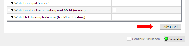
The parameters required to run the solver are located on the Stress tab (see the figure below).
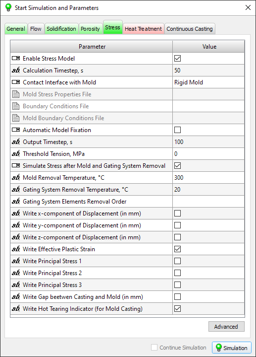
The Hooke solver has many parameters that allow the user to control flexibly the work of the solver. These parameters are not simulation parameters, so they are not on the Stress Tab. To access the solver settings, click the Advanced button on the Stress Tab (see the figure below).
The button opens the preprocessor settings window in the Stress Model section (see the figure below). There are many solver parameters that are grouped in a different tabs.
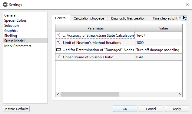
In general, you may not change these parameters and use the default values, which in most cases will be optimal. However, getting the experience with the Hooke module, the user can look at the processor settings to have an access to the additional (advanced) capabilities of the solver.
The stress-strain state of the casting at the end of solidification is due, in general, to the history of the temperature field change of the casting and its contact with the mold. This condition is not final, and can significantly differ from the stress simulation of the casting demolded and cleaned from the elements of the gating-feed system (GFS). Thus, in order to understand what the final geometry of the casting will be and how the residual stresses will be distributed in it, it is necessary to simulate the stress after removing the casting block from the mold and then after removing the GFS elements. The Hooke solver provides necessary functionality for this.
The parameters responsible for the stress simulation at the technological stages, after the casting has solidified, are set on the Stress tab. The Simulate Stress after Mold and Gating System Removal parameter enables the additional Stress simulation at the stages of demolding and removal of the gating system.
The extraction of the casting block from the mold is carried out at a certain point in time or at a certain temperature. For the correct modeling of the stress during the demolding, the dynamics of the change in the temperature field of the casting is important first of all. Therefore, the simulation closest to the actual situation can be performed if the *.cst temperature field file simulated in the Fourier solver contains a complete history of temperature changes in the casting nodes from the beginning of solidification to the point of extraction from the mold. However, in the most cases, the demolding of the casting block from the mold occurs at the temperatures that are well below the solidus temperature, and sometimes at ambient temperature. Then, the simulation of the cooling down to the room temperature will take a long time, the casting temperature files (*.cst), the mold (*.mld) and others will be quite large. To avoid such a situation, the Mold Removal Temperature parameter sets the average temperature of the casting when it is removed from the mold. Using this parameter allows you to do the solidification simulation in the Fourier solver as usual, to the solidus temperature. When simulating in the Hooke solver, first the stress of the casting (with or without the mold) is simulated by the temperature fields from the *.cst file (until the last moment of time), and then the stress of casting without a mold is simulated at the temperature specified by the indicated parameter. The task of searching the temperature fields and the time required to achieve this average temperature is not considered here. If to set the parameter Mold Removal Temperature to a "-1" value, the simulation of the stress of the casting block upon demolding will be made on the basis of the temperature field saved in the last simulation step in the *.cst file.
At this stage the results of the stress simulation are saved in a separate file *_MLDREM.nds. If the creation of the additional files is enabled on the "Show the additional fields" tab in the solver settings, they will also be created when simulating this stage. The names of the additional files will have a "_MLDREM_" prefix.
Note: Stress simulation after the demolding of the block from the mold is carried out only if the contact interaction of the casting with the mold is switched on. With the contact interaction turned off, the stress simulation after the block is removed from the mold is not performed.
Cutting off elements of the gating-feed system usually occurs at ambient temperature. However, the user can set a different average casting temperature for this operation using the Gating System Removal Temperature parameter. The temperature of the casting varies step-like from the temperature of demolding to the temperature of the gating-feed system cutting of. The case of searching the temperature fields and the time required to reach this average temperature is not considered here. If to set the Gating System Removal Temperature parameter to a "-1" value, the simulation of the stress will be made on the basis of the temperature field saved in the last simulation step in the *.cst file.
The separation order of the gating-feed elements from the casting is specified by the Gating System Elements Removal Order parameter. The indices of the separated volumes are specified via a space in the required order. It means that the gating-feed elements, the removal of which is planned to be simulated, should be assigned the separate volume indices in advance (except 1). The casting itself must have a volume index of 1. This is done in the Master module before simulating the temperature field in the Fourier solver. If the parameter is specified by an empty line, the stress simulation after gating-feed system elements cutting off will not be performed.
At this stage, the results of the NDS simulation are saved in a separate file *_REMx.NDS, where x is the indices of the deleted volume. If writing additional fields to *.u3d files is enabled, they will also be created when simulating this stage for each deleted volume. The names of the additional files will have a prefix "_ REMx _".
Note: The files containing the gap field between the casting and the mold (*_gap.u3d and *_gap_mm.u3d) are not recorded when simulating the stress at the stage of mold and gating-feed system elements removal.
This section contains the brief data of the simulation methods of stresses and deformations used in the Hooke solver. More detailed can be found in the followings publications:
and other.
The simulation of stress, appearing at the moment when the casting is cooled, is made on the basis of the theory of small elastoplastic deformations created by AA. Ilyushin (see, for example, [1]) using the linear finite element (FE) approximation on the unstructured tetrahedral meshes. The FE approximation of the elastoplastic task leads, at each step of the simulation, to a system of nonlinear equations with respect to the components of the nodal movements. To solve this system, the Hooke solver uses the Newton's method (for example, see N.S. Bahvalov, N.P. Zhidkov, G.M. Kobelkov. Numerical methods – third edition. – M.: BINOM. The laboratory of the knowledge, 2004).
The Newton’s method has a high rate of iterations convergence, but it requires a good initial approximation to the solution. In case if the initial approximation is far from the solution, the convergence may be violated (moreover, the iterative process may begin to diverge, which will be accompanied by a catastrophic increase in the error of the solution).
At each step of the simulation, the movement field, simulated in the previous step, is taken as the initial approximation of Newton's method. Thus, the quality of the initial approximation will be determined by the "proximity" of the movement fields corresponding to the current and previous steps of the simulation. This is crucially influenced by the rate of change in time of the input data of the task (the temperature fields and physical-mechanical properties of the environment) and the magnitude of the time step. When you manually select the value (Use Variable Time Step parameter is disabled) of this step, you should guide how intensively these data change over time. Using the variable time step (Use Variable Time Step parameter is enabled) allows to automate this process: in this case, the step is selected automatically according to the set restrictions on the values of the time variation of the input data of the task. In the case if the magnitude of the time step is set too large, or the limits of the rate of change in the time of the input data of the task are set unsuccessfully, the convergence of the Newton’s method may be violated. The Hooke solver indicates that the application of the Newton’s method is failed, if either the magnitude of the discrepancy value of the system increased monotonically on three consecutive iterations, or if the required accuracy of the solution (set by the Required Accuracy of Stress-strain State Calculation parameter) was not reached after the maximum allowed number of iterations of the Newton’s method (set by the Limit of the Newton's Method Iterations parameter). In the case of such a situation, the initial approximation for the Newton’s method at the next step of the simulation (which is taken as the movement field simulated at the current step) can be too rough, and the application of the Newton’s method may fail again. Thus, the "unsuccessful" application of the Newton's method at any step of the simulation, as a rule, leads to "spoilage" of the rest of the simulation. Therefore, after the first "failure" of the Newton's method, an emergency completion of the simulation is performed. After the emergency termination, you can, for example, specify the other simulation parameters (reduce the time step size, or set more stringent limits on the rate of change of input data) and try to restore it based on the data of the state file.
When simulating the stress for the initial time, a zero movement field is taken as the initial approximation of the Newton’s method, which corresponds to a homogeneous temperature field in the absence of the external loading and plastic deformations. For this reason, to ensure the convergence of the Newton’s method, it is desirable to start the simulation from a homogeneous temperature field (or close to that).
Note: Starting with the version 13.4, the Hooke solver uses the modified Newton’s method, which is characterized by higher stability and much less demanding for the quality of the initial approximations.
When simulation the stress of the casting without taking into account the contact interaction of the casting and the mold, it is necessary to set the special boundary conditions for some mesh nodes - the fixing conditions (FC). The purpose of the setting the FC is to exclude the possibility of shifting the entire cast as an absolutely rigid body. Otherwise, the task turns out to be undetermined, and the movement field acquires a certain degree of arbitrariness (the corresponding elastic-plastic task has an infinite set of solutions). In particular, this can lead to the fact that at each step of the simulation the part will be moved or rotated in an unpredictable manner, or even to the impossibility of the stress simulation on individual simulation steps.
The FC setting can be performed either automatically or manually; the corresponding mode is determined by the value of the parameter Automatic model fixing. When automatic setting of FC (Automatic model fixing parameter is enabled), the number and spatial configuration of the symmetry planes are taken into account of the task under consideration. The constraining of the additional restrictions on any nodes of the casting is not allowed.
When manually setting the FC nodes (Automatic model fixing parameter is disabled), the correct setting of these conditions is entirely the user's responsibility, since an automated check of the correctness of the setting of these conditions is not possible. When specifying these conditions, it is necessary to take into account the number and spatial arrangement of the symmetry planes of the task under consideration (see below). However, it should be noted that in the presence of the symmetry planes that are not parallel to the coordinate planes, in general, it is impossible to correctly determine the FC task, since in this case it is necessary to limit the movements of the individual model nodes along the directions other than the coordinate axes.
Setting of the FC including with the use of the automatic fixation of the model in space, is not allowed in the stress simulation considering the contact interaction of the casting and the mold. This is due to the fact that the FC implied on the casting can conflict with the geometric constraints on the contact boundaries, in the result of which the simulated fields can acquire the nonphysical distortions.
Important! The nodes fixing that are not on the surface of the body is not allowed.
The conditions for the nodes fixation are specified in the Mirage module and saved to the mcst file (see the section Creating the boundary conditions files for the stress simulation). The number of the fixed nodes cannot exceed five thousand.
In case if the considered thermoelastoplastic task does not have any plane of symmetry, then the movement field is determined to within an arbitrary movement of the entire model as an absolutely rigid body, that is, the model has six degrees of freedom. For this case, there is a traditional scheme of imposing the restrictions on 3 casting nodes (see the figure below), the application of which completely excludes the arbitrariness in determining the movement field. Its meaning is that, despite the fact that all six degrees of freedom of casting are limited, there is no obstacle to the movement of its individual nodes (with the exception of one node). As a result, a reliable stress field without peak values at the fixing nodes is obtained.
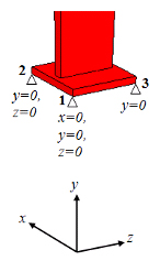
Consider the proposed scheme. The first node is prohibited from moving across all three axes. This restriction fixes three degrees of freedom of the casting (moving along the axes x, y, z). The second node is moved relative to the first along the x-axis (the orientation of the fixed nodes relative to the coordinate axes is important), it is prohibited to move along the vertical axis (fixing the casting rotation around the z-axis) and along the axis perpendicular to the segment node1-node2 (prohibition of the casting rotation around the vertical axis). At that, the second node can move freely along the x-axis. And, finally, the third node fixes the last degree of freedom - prohibits the rotation of the casting around the x axis.
Let us consider the possible schemes of a "manual" setting of FC in the case of the presence of symmetry planes. It is necessary to distinguish the following cases:
These cases are characterized by a different number of the degrees of freedom, and, as a consequence, the various schemes for fixing the nodes.
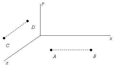
The case of one symmetry plane. For the clearness let the plane of the symmetry be the plane y = 0 (see the figure below). Then, due to the symmetry of the movement field with respect to this plane, the component uy of the movement field becomes zero on this plane. This circumstance excludes the rotations around any axes parallel to the coordinate axes Oz and Ox, as well as moving the entire body as the absolutely rigid along the direction of the Oy axis. Thus, the number of the degrees of freedom is reduced to three: the movements of the body are possible as the absolutely rigid in the directions of the axes Oz and Ox (i.e. parallel to the plane of the symmetry) and the rotations of the body around a certain (arbitrarily chosen) axis parallel to the Oy axis. It is possible to fix these degrees of freedom by imposing the following additional conditions on the movement field. Let’s take an arbitrary segment AB parallel to the Ox axis (see the figure below). At the A node, we set uz = ux = 0 (which fixes the translational degrees of freedom), and at the B node - uz = 0 (which fixes the remaining rotational degree of freedom). We can achieve the same result in the following way: taking an arbitrary segment CD parallel to the Oz axis, at the C node we require uz = ux = 0, and at the D node - ux = 0.
The case with two intersecting symmetry planes.For clearness, let the planes z = 0 and x = 0 be the planes of symmetry. In this case, under the conditions: uz = 0 for z = 0 and ux = 0 for x = 0, only one degree of freedom remains: the movement of the body as the absolutely rigid in the direction of the line of intersection of the planes of symmetry (that is, the Oy axis). In order to fix this degree of freedom, it is enough to put uy = 0 in one arbitrarily chosen node. In the general case, that is, when there are two intersecting symmetry planes oriented in a space in an arbitrary manner, it is necessary to require that the projection of the movement vector to the direction of the intersection line of these planes vanishes at some nodes.
The case with three intersecting symmetry planes. There are possible two situations:
In fact the case a) does not differ from the case of two intersecting planes of symmetry already considered. In the case b) all six degrees of freedom of the body are fixed, and no additional conditions imposing on the movement field is not required.
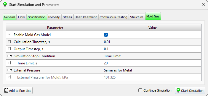
The mold gas flow analysis is performed by the Fourier solver in conjunction with the casting solidification calculation. When the integrated gas flow model is activated during the calculation, two files will be written in addition to the other results:
Taking into account the observed pattern of gas formation and removal, decisions can be made on adjusting the technology, venting the core or mold, regulating the density to increase gas permeability, etc.
When setting up a calculation that includes an analysis of the mold's gas regime, it is necessary to specify parameters describing the solidification conditions and parameters on the Mold Gas tab (see the figure below).
The casting macrostructure is modeled on a 2D mesh of a cellular automaton (CA) with a square cell.
The simulation uses temperature fields calculated in the Fourier module on a finite element mesh (FE). To represent the temperature fields, the CA cells are grouped into blocks of the same size. The choice of block sizes depends on the temperature gradient in the selected section of the casting. Usually, the block size is at least 10x10 cells.
The nucleation and growth of grains occurs in the casting mushy zone. The dimensions and configuration of the mushy zone change over time. Therefore, in the modeling of the macrostructure at each moment of time, only a part of the CA blocks participate, which in the course of the calculation can become active for a while and then be excluded from the calculation.
To organize this process, CA blocks are united into local computational domains (LCD), which are connected to the calculation and removed from the calculation, depending on whether they have active blocks.
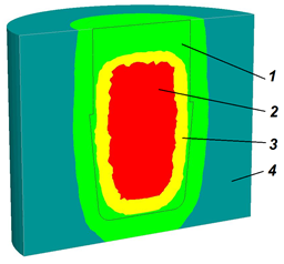
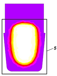
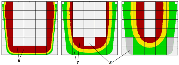
The casting macrostructure is modeled using temperature fields calculated in the Fourier thermal solver on a FE mesh. When the structure solver is launched, the temperature fields are processed and transferred from the finite element mesh to the cellular automaton mesh. As a result of this processing, the temperature distributions for the selected section of the casting are extracted from the *.cst file, and a temperature history file (*.tbl) is formed, recorded for the CA blocks (see a, b in the figure below).
At the stage of creating a tbl-file, a global computational domain (GCD) is formed, which includes the selected area of the casting.
Simultaneously with the temperature history file, a mask file (*.flags) is created containing information about the boundaries of the area where the casting alloy is located. The file marks local computational domains (LCD) containing metal and LCD, located outside the casting and not participating in the calculation, as well as boundary blocks located at the of casting-environment and casting-mold boundaries . Based on these data, a file (*_temper_loc.fld) is created, which contains fragments of the temperature distribution for LCD that are active at a given time (see in the figure с below).
 |
 |
a |
b |
 |
c |
Dividing the selected section of the casting into local computational domains allows optimizing computational resources and reducing the computation time. LCD become active when the temperature in at least one of the blocks drops below the liquidus temperature. LCD become inactive when the temperature in all blocks becomes less than the solidus temperature.
The number and dimensions of LCA and the sequence of their activation and deactivation are automatically determined by the solver based on the geometry and the selected casting section.
As a rule, metal alloys in the solid state have a body-centered or face-centered cubic crystal cell.
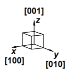
Initially, the solid phase nucleus has a shape close to spherical, however, the anisotropy of the growth of the crystalline material very quickly affects and the nucleus acquires the shape of a cube. In the coordinate system associated with the nucleus and oriented along the edges of the cubic crystal cell, these growth directions (i.e., the normals to the faces) are denoted as [100], [010], [001] (see Fig. a below). In case of the cubic crystal cell, the faces of the cube have the maximum growth rate. All these directions are equal, so we say that a nucleus with a cubic crystal cell grows along directions of the [001] type.
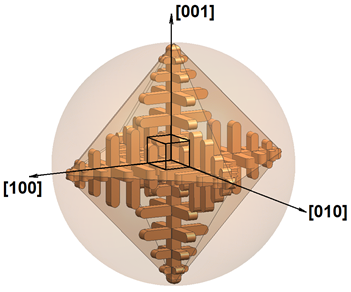
The growth anisotropy leads to the fact that the cubic nucleus very soon takes the form of a dendrite. A freely growing dendrite in a supercooled melt with a uniform temperature field has the shape of a three-dimensional cross with six primary arms (trunks) of growth. As the primary arms grow, their surface loses stability and secondary branches form on it. They also grow in directions like [001], i.e. perpendicular to the primary arms (see fig. b below).
 |
 |
a |
b |
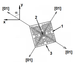
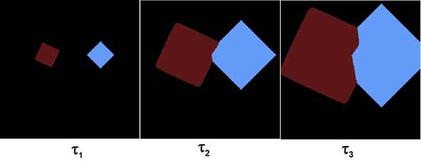
In the 2D approximation, a grain growing in a uniform temperature field has four first order arms of the [01] type of equal length. On fig. below, the grain is shown in the (X, Y) coordinate system associated with the casting. The grain has a random orientation in space, which is characterized by the angle a between the nearest vector [01] and the Y axis. The lines connecting the vertices of the primary arms form an encircling figure that outlines the boundaries of the space occupied by the grain. In a uniform temperature field, all primary axes grow at the same rate and, therefore, the grain enclosure is a square. The correct shape of the enclosure is realized only under conditions of a uniform temperature field. The presence of a temperature gradient leads to different growth rates of primary dendrite arms, which distorts grain boundaries. With the growth of many grains, their growth stops when they collide with neighbors, which also violates the correct shape of the grain.
To simulate the growth of a solid-phase nucleus with a cubic crystal cell, the cellular automaton method is used. It is well known that CA have anisotropy of properties. The anisotropy of CA leads to the fact that, if special measures are not taken, cubic nuclei with an arbitrary orientation lose their original orientation after three generations.
The model implements a growth algorithm that does not require grain shape adjustment. The cellular automaton rules are based on the following principle. Having built a dendrite environment of scale t1, on the field of the cellular automaton, at the next step we can obtain a similar figure of scale t2 = t1 + Dt by constructing a set of figures of scale Dt at each point of the current figure. n this way, consistent grain growth from smaller to larger scales can be ensured. The current time is used as the scale, and Dt is the time step for solving the growth problem.
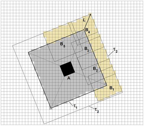
The figure below shows the algorithm for changing grain size A of a square shape rotated at some angle relative to the CA grid in a uniform temperature field. The gray color shows the CA cells located within the boundaries of grain A, i.e. inside the line marked as t1 = const. Since t1 is the current process time, the grain boundary is a constant time line. Let us assume that at the next time step, under conditions of a uniform temperature field, the grain boundaries should represent a similar figure - a square with a half-diagonal, the length of which increased by segment L. The length of this segment depends on the growth rate of the primary dendrite axes and the time step Dt. The new boundary t2 = const is obtained by constructing a set of new type B grains on the boundary gray cells of the CA (only some grains В1 – В5 are shown in the figure below).
For the correct display on the CA mesh of figures of scale Dt (type B), it is necessary that the number of cells representing these figures on the CA mesh be sufficiently large.
The optimal time step for solving the growth problem is defined as:
|
(1) |
| where V – growth rate of the primary dendrite arms; h – CA cell size. |
Empirically, it was found that the shape and orientation of the square when expanding its boundaries is not lost if the length of the segment L is 4-5 cells. On fig. below the result of simulation of the growth of two grains of arbitrary orientation in a uniform temperature field is shown, demonstrating the absence of dependence of the simulation results on the CA mesh.
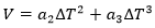
The growth rate of the primary dendrite arms depends on the current undercooling of the melt:
|
(2) |
| where a2, a3 – coefficients determined by the chemical composition of the alloy; DT = TL - T – undercooling of the melt; TL, T – the liquidus temperature of the alloy and the current temperature of the melt at the top of the primary dendrite arm respectively. |
This model assumes heterogeneous nucleation of grains, both on the surface of the mold and in the volume of the melt.
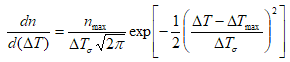
The solid phase nuclei formation occurs almost instantaneously when critical undercooling is reached. Random deviations in the nucleation process are described by the Gaussian distribution:
|
(3) |
| where n – the density of the solid phase nuclei; nmax – density of possible nuclei, 1/m3; DTmax – average undercooling at the the solid phase nucleation, °C; DTs – standard deviation, °C (see figure below). |
In the interval 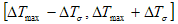 the nucleus formation probability is p > 0.68.
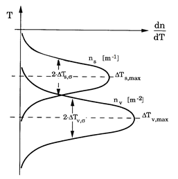
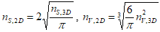
The maximum density of nuclei is limited by the size of the CA mesh. It is assumed that only one solid-phase nucleus can form in a CA cell. Therefore, the density of nuclei that can potentially arise in the volume of the melt must satisfy the condition 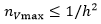 , where h – is a CA cell size. Accordingly, at the “casting-mold” boundary
  .
.
Gaussian distribution characteristics (3) - average undercooling DTmax, standard deviation DTs and nucleus density nmax an only be determined experimentally. It should be taken into account that the experimental data on nmax can refer to a three-dimensional casting. The values for the 2D section of the casting are obtained from the following stereological relations:
|
(4) |
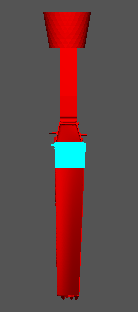
The parameters required to run the solver are on the Structure tab (see figure below). The parameters for the grain growth model are also required (see Equation 2 in the Grain Growth Model section). They are set in the material editor (see the Grain Growth Tab section for more details).
Below are the parameters required for the solver, they are divided into the following groups:
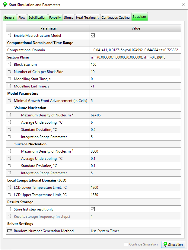
 located at the end of the line. After that, the parameter line will display the coordinate ranges of the selected area, and the area will be selected by the described box (see the figure below). If the parameter is not set, the temperature field of the entire casting will be considered.
 |
 |
a) |
b) |
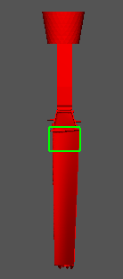
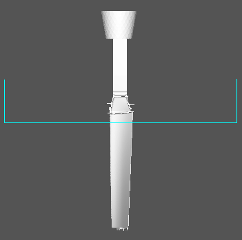
Attention. The structure calculation is possible only in the section orthogonal to one of the coordinate axes. If you try to specify a section of arbitrary orientation, the line will be colored red and it will be impossible to start the calculation.

Usually, the Fourier thermal solver calculates the temperature field starting from the moment the mold is filled until the casting is completely solidified. To model the structure in a selected region (section), it is necessary to have a temperature field in this region from the moment the liquidus temperature is reached to the moment the solidus temperature is reached. This time range can be substantially narrower than the total solidification time of the entire casting. The correct choice of the time range significantly reduces the size of the saved files and the calculation time. If the macrostructure calculation is performed separately from the thermal calculation, the necessary values can be determined in the Mirage postprocessor by analyzing the temperature fields in the desired area of the casting.
The appearance of solid phase nuclei in a supercooled melt is a random process. The number of nuclei that appear in the melt when the supercooling changes by a small d(ΔT) value is described by the Gaussian distribution (3). The parameters of solid phase nucleation are set separately for the melt volume and for the casting-mold interface (for the surface nucleation parameters, see the Surface Nucleation section).
In the presence of large temperature gradients, a high rate of melt cooling, and/or an unreasonably large time step for calculating the thermal problem, errors in the automatic processing of the LCD are possible. To prevent this situation, the user is given the opportunity to independently determine (extend) the temperature interval for the existence of LCD using the following parameters.
The structural and mechanical properties models in the Heat Treatment module are suitable both for cast and deformable steels and can be used to simulate the following types of heat treatment: annealing, normalizing, quenching and tempering.
Heat treatment processes calculations are based on a group of models that allow to predict the microstructure and properties. The appropriate model that meets the required accuracy criteria may be selected by user. Basic models for calculating the microstructure and hardness are supplemented with original statistical models for predicting the tensile strength, yield stress and elongation.
Available models are divided into two groups according to their application field:
Creusot-Loire model was developed in the Creusot-Loire laboratory. That is a statistical model developed on the basis of data processing of test results for samples used in experiments for plotting the continuous cooling transformation (CCT) diagrams of austenite decomposition for low-alloy steels of different chemical compositions at different austenitizing conditions [1, 2]. The application of the model is based on the following assumption: for the same chemical composition, at equal austenitizing conditions and equal cooling rates in the range of 800-500 °C, the resulting microstructures and properties are equal in the sample which has been analyzed for plotting the CCT diagram and in the certain point of the real part.
The hardenability model is based on a comparison of the cooling rates in the range of 800‑500°C in a standard hardenability test specimen (EN ISO 642) and in the specific FE mesh node which belongs to the analyzed part. As in the Creusot-Loire model, it is assumed that if the rates are equal, then the resulting microstructures and properties are also equal for steel of the same composition at the same austenitizing conditions.
The general principles of GPBM are follows:
For the one calculation cycle of heat treatment with polymorphic austenite transformation, only one model of austenite decomposition can be selected. In case the subsequent tempering is included to the heat treatment procedure for the part, then in addition to the austenite decomposition model, one of the available tempering models can be selected. The table below shows compatibility of the austenite decomposition and tempering models included to the software. At the preprocessing stage, during making settings for the calculation, the compatibility of models is automatically controlled in the appropriate Start Simulation and Parameters window.
| Table.Compatibility of austenite decomposition and tempering models |
| Austenite decomposition model | Tempering model | ||
| Creusot-Loire | Spies | Just | |
Creusot-Loire |
+ |
|
|
Hardenability-based |
|
+ | + |
GPBM |
+ |
|
|
To perform calculations of the microstructure and properties obtained after cooling from the austenitizing temperature, it is necessary to specify the following initial data for austenite decomposition models:
The calculation of microstructure and properties is performed together with the calculation of the cooling of the part according to the specified heat treatment regime. It is necessary to set the austenitizing temperature as an initial (the part is considered as uniformly heated). The cooling rates required for predicting the results of heat treatment will be calculated based on the data obtained when solving the thermal problem.
The result of the calculation using the austenite decomposition model will be the following set of data:
To calculate properties after tempering the following additional data are required:
The result of the tempering calculation will be the following data set:
The Heat Treatment model is integrated into the Fourier solver and can be used by the user when setting the appropriate calculation problems. The figure below shows a diagram of the heat treatment model operation coupled with thermal analysis performed by the Fourier solver.
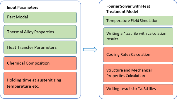
After the calculation is completed, in addition to the temperature field file with cst extension, universal format files with u3d extension, containing heat treatment simulation results, will be written. The table below explains the indication of the name of the result files that will be written on hard disk after the calculations of the heat treatment with austenite transformation, as well as (if necessary) the subsequent tempering is finished.
| Table. File names with heat treatment calculation results for different models |
| Result file | The value field written to the file | Austenite decomposition models | ||
| Creusot-Loire | Hardenability | GPBM | ||
*_ht_crs.u3d |
Cooling rate (°C/s) |
+ | + | + |
*_ht_fp.u3d |
Volume fraction of ferrite-pearlite mixture (%) |
+ |
|
+ |
*_ht_f.u3d |
Volume fraction of ferrite (%) |
|
|
+ |
*_ht_p.u3d |
Volume fraction of perlite (%) |
|
|
+ |
*_ht_b.u3d |
Volume fraction of bainite (%) |
+ |
|
+ |
*_ht_m.u3d |
Volume fraction of martensite (%) |
+ | + | + |
*_ht_au.u3d |
Volume fraction of austenite (%) |
|
|
+ |
*_ht_hv.u3d |
Vickers hardness (HV) |
+ |
|
+ |
*_ht_hrc.u3d |
Rockwell hardness (HRC) |
|
+ |
|
*_ht_uts.u3d |
Tensile strength (MPa) |
+ | + | + |
*_ht_ys.u3d |
Yield stress (MPa) |
+ | + | + |
*_ht_elong.u3d |
Elongation (%) |
+ | + | + |
| Table. File names with tempering calculation results for different models |
| Result file | The value field written to the file | Tempering model | ||
| Creusot-Loire | Just | Spies | ||
*_ht_t_hv.u3d |
Vickers hardness (HV) |
+ |
|
|
*_ht_t_hrc.u3d |
Rockwell hardness (HRC) |
|
+ |
|
*_ht_t_hb.u3d |
Brinell hardness (HB) |
|
|
+ |
*_ht_t_uts.u3d |
Tensile strength (MPa) |
+ | + | + |
*_ht_t_ys.u3d |
Yield stress (MPa) |
+ | + | + |
*_ht_t_elong.u3d |
Elongation (%) |
+ | + | + |
Each heat treatment analysis generates a relatively large number of result files in u3d format. For easing the navigation, all of them will be written to a separate subfolder inside the project folder. The name of this subfolder for heat treatment calculation result files will be formed in such a way that it can be used for recognizing the enabled models of austenite decomposition and (if applicable) tempering. The principles of indexing the names of the subfolders are given in the table below.
| Table. Names of folders with calculation results depending on the selected austenite decomposition models and tempering models |
| Austenite decomposition model | Tempering model | |||
| No | Creusot-Loire | Spies | Just | |
Creusot-Loire |
HT-CL |
HT-CL_T-CL |
|
|
Hardenability-based |
HT-HRD |
|
HT-HRD_T-SP |
HT-HRD_T-JU |
GPBM |
HT-PhB |
HT-PhB_T-CL |
|
|
When running a new calculation for a project with the same name, the heat treatment models may be enabled in a new combination. The previously written subfolder with the saved results from the last heat treatment calculation will be deleted and replaced with a new one after the calculation is started again.
The searching process of optimal technological solution may require a series of calculations to check changes of the part cooling conditions, varying the holding time, etc., as well as using of different models for predicting the treatment results. To prevent the mix-up and data loss when performing such calculations, it is strongly recommended to save g3d project for each new version of the analysis under the new name in the separate new folder.
The models underlying the module are designed to analyze heat treatment processes, including heating to the austenitization temperature and subsequent cooling down to ambient temperature, as well as heating and holding for high tempering. Using the model, the structure and properties after annealing, normalization, quenching, quenching followed by tempering, some cases of surface quenching, etc. can be assessed.
The models are not intended to predict structure and properties for heat treatment processes that include interrupted cooling. Calculations cannot be made for such technologies as interrupted quenching, quenching with self-tempering, and isothermal quenching. However, GPBM can be used to calculate the microstructure and properties for heat treatment process that includes isothermal holdings during the cooling stage.
Solving of the thermal problem along with austenite transformation can be carried out for low-carbon, medium-carbon and low-alloyed steels with the content of alloying elements according to the table below.
| Table. Allowed contents of chemical elements |
| Element | Content limits for different models, % | |||||
| Creusot-Loire | Hardenability-based | GPBM | ||||
| Standard | Extrapolation | Standard | Extrapolation | Standard | Acceptable | |
| C | 0.10-0.50 | 0.05-0.58 | 0.10-0.70 | 0.01-0.90 | 0.05-0.58 | 0.01-0.80 |
| Si | ≤1.00 | ≤1.00 | 0.15-0.60 | 0.01-2.00 | ≤1.37 | ≤3.50 |
| Mn | ≤2.00 | ≤2.00 | 0.50-1.65 | 0.01-1.95 | ≤2.00 | ≤2.00 |
| Ni | ≤4.00 | ≤4.00 | ≤1.50 | ≤3.50 | ≤4.00 | ≤8.50 |
| Cr | ≤3.00 | ≤3.00 | ≤1.35 | ≤2.50 | ≤3.00 | ≤13.00 |
| Mo | ≤1.00 | ≤1.00 | ≤0.55 | ≤0.55 | ≤1.00 | ≤4.50 |
| Cu | ≤0.50 | ≤1.00 | ≤0.35 | ≤0.55 | ≤1.00 | ≤1.50 |
| Al | 0.01-0.05 | 0.01-0.05 | ≤0.05 | ≤0.06 | 0.01-0.05 | ≤1.00 |
| V | ≤0.20 | ≤0.50 | ≤0.20 | ≤0.20 | ≤0.27 | ≤2.00 |
| Zr | 0 | 0 | ≤0.25 | ≤0.25 | 0 | ≤0.25 |
| B | 0 | 0 | ≤0.005 | ≤0.005 | 0-0.028 | ≤0.03 |
| Nb | 0 | 0 | 0 | 0 | 0 | ≤0.55 |
| Ti | 0 | 0 | 0 | 0 | 0-0.12 | ≤0.45 |
| W | 0 | 0 | 0 | 0 | 0-2.25 | ≤18.00 |
| Mn+Ni+Cr+Mo | ≤5.0 | ≤6.0 | - | - | ≤5.9 | ≤5.9 |
If the chemical composition of the steel lays within the range of standard values (different for different models), increased calculation accuracy can be ensured. If it goes into the extrapolation or permissible values range, the calculation of the microstructure and properties can still be performed with satisfactory accuracy. In case the chemical composition is outside the range for the selected model, the calculation cannot be started.
When using GPBM, the calculation of the structure and properties is possible only if the chemical composition of the steel lays within the range of normative values; if it goes into the range of permissible values, only the microstructure will be calculated.
The permissible range of temperature-time parameters of tempering when calculating according to the relevant models, as well as restrictions on chemical composition, are presented in the table below. The tempering calculation will be performed even if the specified limits of element content are exceeded, with a warning about using the model in the extrapolation area, while going beyond the specified temperature-time parameters is impossible.
| Table. Allowed contents of chemical elements |
| Element | Content limits for different models, % | ||
| Creusot-Loire | Spies | Just | |
| C | 0.05-0.58 | 0.13-1.15 | |
| Si | ≤ 1.00 | 0.06-1.62 | |
| Mn | ≤ 2.00 | 0.30-1.90 | 0.30-1.67 |
| Cr | ≤ 3.00 | ≤ 1.54 | |
| Ni | ≤ 4.00 | ≤ 3.03 | |
| Cu | ≤ 1.00 | ≤ 0.23 | |
| Mo | ≤ 1.00 | ≤ 0.26 | |
| V | ≤ 0.50 | ≤ 0.10 | |
| Mn+Ni+Cr+Mo | ≤ 6.00 | - | |
| S | - | ≤ 0.03 | |
| P | - | ≤ 0.035 | |
| W | - | ≤ 0.01 | |
| Ti | - | ≤ 0.04 | |
| Al | - | ≤ 0.035 | |
| Sn | - | ≤ 0.01 | |
| B | - | ≤ 0.002 | |
| N | - | ≤ 0.01 | |
| Table. Acceptable values of model parameters |
| Parameter | Value ranges for different models | ||
| Creusot-Loire | Spies | Just | |
| Tempering temperature, °C | 500-700 | 100-700 | |
| Holding time at tempering temperature, h | 1-200 | 0.1-24 | |
The structural components "ferrite" and "pearlite" in the results of simulation with Creusot-Loire model are not separated and their individual ratios are not available. When using the model based on hardenability, only data on the martensite volume fraction are available among the structural components. The Creusot-Loire and GPBM models do not separate different bainite morphologies.
At the beginning of the calculation, the part is considered to be heated uniformly: all mesh nodes have the same temperature and the same thermal history. The isothermal holding time at the austenitizing temperature is set by the user.
The calculation of the tensile strength is carried out according to known dependencies based on the obtained Vickers hardness values. Yield stress and elongation values are calculated using statistical models built on the basis of data from mechanical tests in production laboratories. The input parameters of these models are the tensile strength values and the chemical composition of the steel.
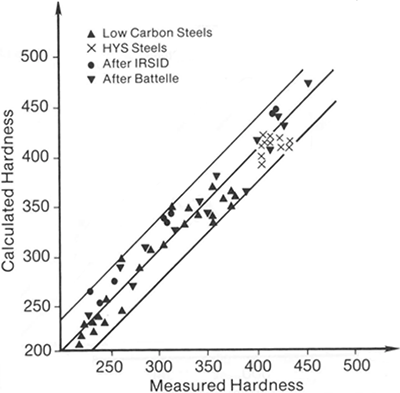
The prediction accuracy characteristics for different HT models, using the median absolute error (MedAE) metric, are shown in the figure below. The estimates were made for the most general conditions of the heat treatment analysis problem, based on data extracted from the thermal conductivity curves (CCT) of various steels, taken from reference literature. Information on the chemical composition and austenitization parameters is not fully available, and the extraction of cooling rate data is subject to error due to the fact that the cooling curves in the CCT are plotted on a logarithmic time scale.
In general, to improve the accuracy of modeling, it is recommended to use the company's statistical data for a specific steel grade (chemical composition, use of appropriate CCT, hardenability curves, etc.).
The practice of analyzing HT conditions using different models is common to specialized modeling packages and aligns well with the specifics of the overall problem. The ability to choose a model offers the following advantages and opportunities in terms of the reliability and accuracy of the obtained results.
When selecting a model based on hardenability, it is necessary that the properties of the alloy contain data on the hardenability curve. The corresponding data are specified in the Hardenability & CCT tab when entering the material properties using the property editor.
When selecting GPBM, it is necessary that the properties of the alloy contain data on CCT diagram. The corresponding data are specified in the Hardenability & CCT tab when entering the material properties using the property editor (for more details see the Hardenability & CCT Tab section).
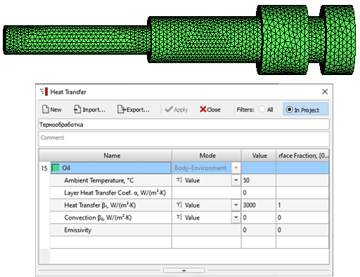
Since the heat treatment analysis uses the temperature history of the cooling of the workpiece, it is necessary to specify all the necessary data for the thermal calculation on the General and Solidification tabs in the Start Simulation and Parameters window (in this case, the name of the Solidification tab should be understood as “Thermal Calculation”). On the fig. below is the Shaft model prepared for heat treatment simulation. Cooling conditions are set as usual at the outer boundary. Depending on the mode, either the default boundary with index 17 (casting-environment) or any other combination of boundaries can be used, for example, if it is necessary to set a variable temperature of the quenching medium, designate air-cooled surface areas, etc.
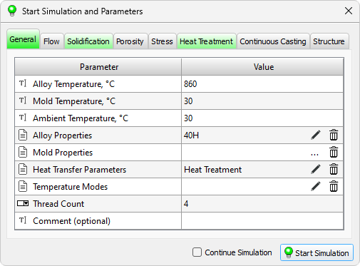
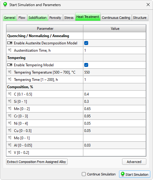
The parameters required to run the Heat Treatment solver are located on the Heat Treatment tab (see figure below).
When click on the Advanced button, which is located under the data table, you go to the solver settings window (see the figure below). It contains special settings for the HT model, which in some cases can be useful for an experienced user.
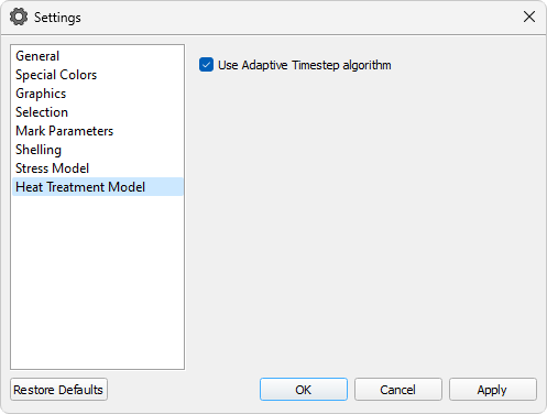
It contains the Use Adaptive Timestep algorithm parameter, which enables automatic control of the calculation step (enabled by default). In this case, the value of the Calculation Timestep parameter on the Solidification tab determines the maximum calculation timestep, which, if necessary, will automatically decreased as the calculation progresses to ensure that the result is obtained with sufficient accuracy. It is recommended to use the adaptive timestep in all cases, keeping the default setting.
There are also additional settings for the adaptive step algorithm. The range of temperature change per calculation step may be adjusted by changing the value of the parameter Max Temperature Change Step. It is preferable to use the default value of 30 °C. When Save all steps option is enabled (disabled by default), a detailed temperature history of the part cooling process will be written in the cst file based on actual calculation timestep, without taking into account the output or calculation timestep specified on the Solidification tab.
The HT solver settings window allows you to disable the automatic correction algorithms for the CCT and hardenability curves based on actual austenitizing conditions (the Hardenability Curve Ajustment and CCT Diagram Ajustment parameters, respectively). In most cases, this automatic correction is necessary and improves calculation accuracy. However, if the user has entered precise data into the editor that fully corresponds to their alloy under the austenitizing conditions used in the problem, this automatic correction introduces error. By default, these parameters are in the "on" state, which is recommended for typical cases.
To calculate the structure and properties, you should click on the Simulation button. The cooling of the workpiece during the heat treatment process and the resulting structure and properties will be calculated.
Note. The calculation of mechanical properties after tempering (if required) is always carried out in conjunction with the simulation of austenite decomposition and cannot be run separately.
As a result of calculations, u3d files with names consisting of the project name and abbreviated names of structural components and properties will appear in the project folder. These files (see figure below) can be opened in the Mirage postprocessor when using the universal format file load dialog.
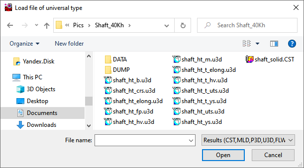
On thr fig. below some results of the calculation of oil quenching of a 600 mm shaft made of 40Cr steel and subsequent tempering at 550°C are shown.
After the parameters of all solvers are specified, you can start the simulation. To do this, click the Simulation button in the lower right corner of the Start Simulation and Parameters window (see the figure below).
Before the calculation is started, the preprocessor Master will require saving all the changes made in the model during the preparation of the calculation. The standard procedure for saving the project will be launched, where the user can specify the folder in which the following will be written:
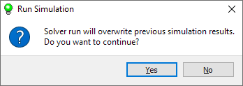
If a project that has already been run for calculation is overwritten on save, a warning message appears indicating that calculation results exist. (see figure below). If you answer Yes, the previous results will be overwritten. If you answer No, the save project will be canceled.
After saving the model, the .bat file will be launched from the calculation folder (the folder where the .g3d file is saved), which is a script for launching the solvers. If desired, the user can edit it independently and start the calculation without the participation of the Master preprocessor.
After starting the calculation, the user sees the console window on the screen, which displays the progress of the calculation. To interrupt the calculation, just close the console.
During the calculation, the results are written to the project folder and can be viewed in the Mirage postprocessor (see the chapter Viewing Results).
If the calculation was interrupted for any reason, it can be continued. When the solvers are running, their current state is constantly written to the DUMP folder, which is created in the project folder when the calculation is first started. When restoring, files from the DUMP folder are read and the calculation continues from the moment it was stopped. In this case, the results are appended to the previously created files.
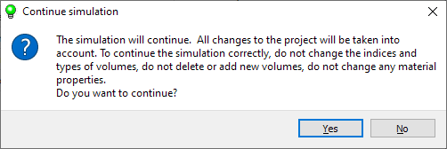
To continue the interrupted calculation, in the Start Simulation and Parameters window, next to the Simulation button, there is the Continue Simulation option (see the figure below). If the calculation is started for the first time, the option is disabled and unavailable for the user. If the calculation was started and then interrupted, the option is enabled and can be used. When the calculation is started with the checked Continue Simulation, it will continue from the time point that was saved in temporary files in the DUMP folder.
It should be note that when restoring an interrupted calculation, changes made to the project will be taken into account. The calculation will continue with new settings and parameters. It is not recommended to change the geometry of the model and the properties of materials, this can lead to malfunctioning solvers and / or unwanted results.
At startup, a message will be displayed (see the figure below) warning about possible changes to a previously started calculation. If you answer Yes, the calculation will continue. If the answer is No, the start of the calculation will be canceled.
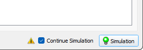
If the Save Calculation State option is turned off in the Master module settings, continuation of an interrupted calculation is possible only from the start of the next solver (see details in Module Settings / General section). For example, if mold filling and then solidification and porosity are simulated, and the calculation is interrupted during the solidification stage, it can only be continued from the beginning of the solidification calculation. This limitation of functionality is indicated by the yellow icon next to the Continue Simulation option (see figure below).
If you unckeck the Continue Simulation option, then when you start the calculation, as usual, you will be prompted to save the project data and the results of the interrupted calculation will be overwritten.
It is possible to run several calculations one after another in batch mode. To do this, you need to write a script and run it in the command window, as described in the example below (for Windows):
cd "calculation A"
call "calculation A.bat"
cd "calculation B"
call "calculation B.bat"
…
In this case, the calculations "calculation A" and "calculation B" must be prepared for launch, i.e. it is assumed that the files "calculation A.bat" and "calculation B.bat" have already been written.
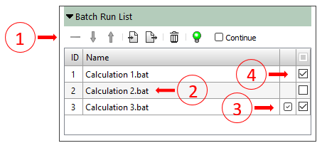
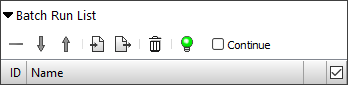
To automate the process of preparing a launch scenario, you can use the Batch Run List panel, which is located under the model tree on the Model Tree tab. (See the figure below). It contains a toolbar (1) and a table with a list of calculations to be launched (2). The user creates a list of calculations (this will be described below). If the calculation has already been launched but has not reached the end, it will be marked with a checkbox (3) with the hint "The calculation will be continued". If for some reason one of the calculations should not be launched when executing the scenario, it can be disabled in the list using the checkbox (4). n the column header there is a checkbox that enables or disables all calculations in the list.
The commands that control batch execution are located on the toolbar above the list of calculations (see the figure below).
 |
The Delete Selected Rows button deletes the selected row or several rows of the table. It is used if you need to delete one or several calculations from the queue. |
 |
The Move row down button moves one selected row one position down. It is used to form the order of calculations. |
 |
The Move row up button moves one selected row one position up. It is used to form the order of calculations. |
 |
The Import Run List button opens a standard dialog for loading a list of calculations from a file with the pbrl extension. |
 |
The Export Run List button opens a standard dialog for writing the list of calculations to a file with the pbrl extension. |
|
The Clear List button removes all calculations from the list. To remove one or more selected calculations from the list, use the button. |
 |
The Run simulations on the list button starts the process of preparing the list for launch and then starts its execution. If the equipment malfunctions during the list execution, the execution of calculations by list can be restored. To do this, check the Continue box before starting the calculations by list. |
The calculation list is formed as follows:
In the standard model available in the POLIGONSOFT, the creation of the pipe shrinkage and macroporosity is associated with the movement of the melt mirror. Moving the mirror is a consequence of feeding the mushy zone. In the standard model of macroporosity, it is assumed that the flow of liquid metal through the solid phase skeleton is unimpeded right up to the overlapping of the flow channels. At the moment when the melt mirror passes through this point of the casting, the formation of the porosity necessarily takes place, regardless of the magnitude of the external pressure.
In the new model, the formation of the porosity occurs at a time when the creation of a new section interface becomes energetically favorable, i. e. when the resultant pressure in the melt, formed from the external pressure, the metallostatic pressure, the capillary pressure and the pressure drop due to the shrinkage, is able to create a new pore. Thus, in the new model, the macroporosity prediction depends on the external pressure and the rate of metal cooling during crystallization. The cooling rate determines the structure of the casting (the grain size and parameters of the dendritic structure) and, thus, the capillary forces that play an important role in feeding the two-phase zone, the formation and growth of the pores.
It should be emphasized that the standard model of the porosity is an extreme case of a new model corresponding to low melt strength at break, high modulus of compressibility of liquid metal and zero surface tension. Under these conditions, the models demonstrate very close results, the differences in which are associated with the modernization of computational algorithms that ensure more accurate observance of the mass balance.
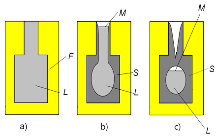
In general, the solidification process of the casting goes through the following stages: the formation of a pipe during the solidification of an open thermal hot spot, the formation of a closed thermal hot spot, the formation of an internal pipe shrinkage or dispersed porosity during the solidification of a closed thermal hot spot (see the figure below).
A thermal hot spot is considered open if the melt is in contact with the surrounding environment (Figure b). In the event that there is no direct contact of the melt with the surrounding environment, the thermal hot spot is considered to be closed (Fig. c).
The solidification of the melt is accompanied by the shrinkage of the metal. In an open thermal hot spot, the solidification does not lead to a drop in pressure, since the shrinkage is compensated by lowering the free surface (or mirror) of the melt. The surface of the melt is able to move, i.e. is free if it does not have a fixed framework of the solid phase formed by the closed dendrites of the growing grains. As in the standard macroporosity model adopted in POLIGONSOFT, a fixed solid-phase framework appears when the fraction of the liquid phase decreases to a critical value fL**, i.e. at fL ≤ fL**.
In the standard porosity model, the movement of the melt mirror in the stationary solid-phase framework leads to dehydration of the interdendritic spaces and the appearance of a porosity numerically equal to the fraction of the liquid phase fL.
In a new model of the porosity, the melt mirror exists only where there is no solid-phase framework, and the interdendritic spaces above the melt mirror are filled with a melt that is retained there due to the capillary effect.
At some point in time, because of the decrease in the fraction of the liquid phase, the boundaries of the thermal hot spot become impermeable, and the thermal hot spot becomes closed (above in the Fig. в). At this point, the free surface of the melt no longer exists in the thermal hot spot and, consequently, the shrinkage of the metal during crystallization is no longer compensated by a change in the position of the mirror. This leads to a decrease in pressure in the thermal hot spot, the intensity of which depends on the modulus of compressibility of the melt E, the shrinkage volume of the metal at a given time step, and the volume of the melt in the thermal hot spot.
It should be noted that, the compressibility modulus of liquids is extremely large (the water is about 2000 MPa). Therefore, in the absence of communication with the environment, the crystallization of the metal leads to a rapid pressure drop in the thermal hot spot to a critical value of Pcrit.
If, at this point, there is a region of melt in the thermal hot spot that is not bound by the fixed dendritic framework (i.e., the region where fL > fL**), a new free surface of the melt appears, which subsequently leads to the formation of a closed pipe shrinkage. If there is no such region, the scattered macroporosity is formed.
In the event when a fixed framework of the solid phase is present everywhere in a closed thermal hot spot, i.e. everywhere fL ≤ fL**, the formation of a flat free surface of the melt is impossible.
Breaking the melt integrity due to the pressure drop occurs by the formation of the macroporosity. The first pore occurs when the pressure drops below the critical value Pcrit. As a rule, the point of origin of the pore is the point at which the pressure is minimal.
After the formation of pores began in the zone, the shrinkage that occurs at each time step is most likely to be compensated by the growth of already existing pores. The growth of the pore depends on the ratio of the capillary forces Pσ = 2σ/r, which tend to close the pore, and the pressure in the melt (see the figure below).
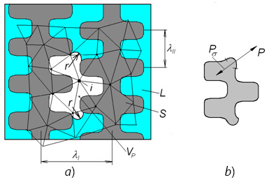
The existence and growth of the pores depend on the equilibrium of forces on its surface, determined by the Laplace equation Pσ = -2σ/r (see the figure below). In this equation, P is the pressure in the melt; σ is the surface tension coefficient; r is the minimum radius of curvature of the pore, determined by the distance between the secondary branches of the dendrites λII, i.e. one of the parameters characterizing the framework of the solid phase.
The formation of the shrink pore occurs when the pressure in the melt drops to a critical value Pcrit, which is determined by the melt strength. In this model only shrink porosity is considered, for the formation of which a tensile stress must appeae in the liquid, i.e. the pressure must be negative.
Based on the surface tension for the nickel and iron melt σ ≈ 1.6 N/m, and the pore diameter observed in the castings 3.5÷ 60 µm, it is evident that the pressure of the melt at the moment of the pore formation can be from -0.1 to -1 MPa.
It is known that the theoretical strength of the melts is very high and can exceed 100 MPa. The actual strength of the melt is much lower and strongly depends on the purity of the metal and the way new interfaces are created, i.e. the pores. It can be assumed that the critical pressure at which the melt integrity is disturbed is within -0.01 - 1 MPa.
The meniscus radius r depends on the size of interdendritic spaces, which are determined by the rate of cooling of the melt in the two-phase zone. When solidification of the shaped castings weighing up to 100 kg, depending on the cooling rate of the melt the possible distance between the secondary dendrite axis constitute 20-100 μm. The distances between the primary axes, or between the grains, are 200 ÷ 600 μm.
The melt compression modulus can be estimated from the formula E = a2ρi, where a is the sound velocity in the melt; ρi is the melt density. Based on the known data on the speed of sound for pure metal melts, we can assume that Е = 3.104 ÷ 105 MPa. It should be taken into account that the sound velocity is much lower in the alloys than in pure metals.
In the model, the compression modulus characterizes the process of pressure drop in the thermal hot spot. Under the ideal conditions, the rate of pressure drop in a closed thermal hot spot is proportional to Е. During the crystallization of a real casting, the solid skin of metal surrounding the thermal hot spot may be permeable, which reduces the rate of pressure drop in the node. There is also the possibility of deformation of the skin under the influence of the difference in the pressures of the environment and inside the thermal hot spot, which also reduces the rate of pressure drop, since a part of the crystallization shrinkage is compensated by the deformation. This indicates that the effective compression modulus of the melt should be much less than the theoretical estimation possibly is equal to 200 ÷ 2000 MPa.
Within the frames of this model, the listed phenomena are not considered, and therefore the compression modulus, like the critical pressure, are the adjustable parameters that must be determined based on the experimental data.
To adjust the model, it is necessary to perform a series of simulations for the existing castings at different values of the parameters Е, Pcrit, σ and λII and to compare the results with the porosity data. In this case, it makes sense to verify the adequacy of the specified thermophysical properties of the alloy and the mold materials, heat transfer conditions, etc., comparing the indications of the thermocouples installed on the casting block with the results of the thermal calculation.
Below there are some reference data on the surface tension for pure metals.
Metal |
Temperature, С |
σ, N/m |
Ni |
1400-1700 |
1,6 |
Ni3Al |
1400-1700 |
1,5 |
Fe |
1400-1700 |
1,65 |
Cu |
|
1.25 |
Au |
|
1,1 |
Pb |
|
0,5 |
Al |
Тmelt÷900о |
0,85 |
Sn |
Тmelt÷350о |
0,53 |


.svg)
.svg)
.svg)

.svg)